05 - Modal Split and Random Utility Model - TDBM

Modal split is the second step in the modeling stage of the classic 4 stage framework.

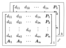
In terms of an O/D matrix like the following, in this step we basically take the matrix, and from that we get 2 ore more (depending on how many option we are looking at).

%%🖋 Edit in Excalidraw%%
where:

$d_{i j} :$ number of trips from TAZ $i$ to TAZ $j$
$P_{i} :$ tot number of trips generated by TAZ $i$
- It's the sum of the colums
$A_{i} :$ tot number of trips attracted by TAZ $j$
- It's the sum of the rows
$n :$ tot number of TAZs
$k :$ the mode of transportation

Along this note, the number of trips from TAZ $i$ to TAZ $j$ will sometimes be indicated with the symbol $t_{i j}$

There are many factors affecting modal choice, some related to passengers (aka characteristics), some to the trip and lastly some variables considered as averages.

Passenger	Trip	Mean
Vehicle availability	Purpose	Waiting time
Income	Hour of the day	Travel time
Family structure		Cost
Housing density		Cost and parking facility
Constraints of the rest of the day		Comfort
		Regularity
		Safety

Discrete choice models

Modal split models are based on utility theory. The general principle is that the trip maker tries to maximize the UTILITY.

utility

Utility is a function that is split into two parts:

$U_{i} = V_{i} + ξ_{i}$
where:

$i = 1. . . m :$ the transport modes
$U :$ the perceived utility
$V :$ the [[#measurable utility]]. Deterministic
$ξ :$ the random part of the utility

Each passenger chooses mode $j$ if

U_{j} = max {U_{i}} \forall i \in I

Given that there is a random part to each utility, it is possible that 2 modes which deterministic utilities are ordered as:

V_{1} > V_{2}

in the end have a perceived utility

U_{1} < U_{2}

due to the random part.

Measurable utility

The measurable utility is a linear combination of attributes:

V_{i} (β, x) = b_{1}^{i} + \sum_{k = 2}^{p} β_{k}^{i} x_{k}^{i}

where:

$β_{i}$ are the parameters to calibrate
$x_{i}$ are the attributes

The parameters are calibrated through the method of maximum likelihood (method of maximum likelihood.

Random utility

The random part of the utility, $ξ$ , needs to be associated to a random distribution if we want to do anything with it.

We can prove that:

\begin{aligned} ξ_{i} & \sim Normal & ⟹ & Probit model \\ ξ_{i} & \sim Gumbel or Weibull & ⟹ & Logit model \end{aligned}

Probit model

The Probit model is particularly useful as it can accomodate for routes that share part of the links.

Logit model

The Logit model is not able to accomodate for routes that share part of the links. In probabilistic terms:

ξ_{i} \sim i.i.d. Gumbel

(i.i.d.: indipendent and identically distributed)

The probability of mode $i$ , given a [[#Measurable utility]] $V_{i}$ and all the other utilities $V_{j}$ , according to the logit model is:

p_{i} = \frac{e^{V_{i}}}{\sum_{j = 1}^{m} e^{V_{i}}}

Nested logit models

The part that follows was written by ChatGPT. I have read it all and it makes sense to me BUT I have used it in place of the slides (since those are terrible and impossible to follow). This mean that I did not get the information from the slides themselves or from any book for that matter.

My understanding of this tipic realies moslty on an explenation provided by Large Language Model and might be inaccurate.

I'd like to add that I hate doing this, as I prefer writing these notes myself and from reliable information but again, the sources I had available were incomprehensible to me I had to choose between understanding something with an unkwon probability of it being correct vs the certeinty of not understanding anything. I chose the first, but I invite anyone reading this to keep this in mind.

🧠 Context

In transportation demand modeling, a modal split model predicts how travelers choose between transport modes (e.g., car, bus, train, bike). This is modeled using discrete choice theory, where each individual picks the alternative that gives them the highest utility.

The classic model is the Multinomial Logit (MNL) model, which assumes:

Perfect substitution between all alternatives.
Independence of Irrelevant Alternatives (IIA) — the ratio of probabilities of choosing two modes does not change if a third one is added or removed.

This is unrealistic when some alternatives are similar" (e.g., bus and train are both public transport), because MNL cannot capture correlation in unobserved factors.

❗ Problem with MNL:

Choosing between car, bus, and train treats bus and train as equally different from car as they are from each other — which is often wrong.

🚦 Solution: Nested Logit Model (NL)

The Nested Logit (NL) model generalizes MNL by allowing for correlation among similar alternatives, while still being computationally tractable.

🌲 Nesting Structure

Imagine the traveler faces this decision tree:

          Travel Mode
         /           \
    Private        Public Transport
     /   \             /      \
   Car  Moto        Bus     Train

Alternatives are grouped into nests based on similarity (e.g., Bus and Train are both PT, and may share unobserved characteristics like comfort or exposure to traffic).

📐 Utility Specification

Each individual $n$ chooses the alternative $j$ that gives the highest utility:

U_{n j} = V_{n j} + ε_{n j}

Where:

$U_{n j}$ : Total utility of alternative $j$ for individual $n$
$V_{n j}$ : Systematic (observed) part of the utility (e.g., cost, time, income effects)
$ε_{n j}$ : Random (unobserved) part

🪜 Nesting and Probabilities

Let's define:

$C$ : the full choice set (e.g., all travel modes)
$B$ : set of nests (branches), e.g., $B = {Private, PT}$
$j \in b$ : alternative $j$ belongs to nest $b$

The probability of choosing alternative $j$ is computed in two steps:

Step 1: Inclusive Value (Logsum)

For each nest $b$ , compute the inclusive value (IV) or logsum utility:

I V_{n, b} = \ln (\sum_{k \in b} e^{V_{n k} / λ_{b}})

Where:

$λ_{b} \in (0, 1] :$ nesting parameter, measuring the degree of independence within the nest:
- $λ_{b} = 1 :$ full independence (ie, back to MNL)
- $λ_{b} < 1 :$ correlation within nest

Step 2: Probability of Nest and Alternative

(a) Probability of choosing nest $b$ :

P_{n, b} = \frac{e^{λ_{b} I V_{n, b}}}{\sum_{h \in B} e^{λ_{h} I V_{n, h}}}

(b) Probability of choosing alternative $j$ within its nest $b$ :

P_{n, j | b} = \frac{e^{V_{n j} / λ_{b}}}{\sum_{k \in b} e^{V_{n k} / λ_{b}}}

🔄 Final Choice Probability:

P_{n, j} = P_{n, b} \cdot P_{n, j | b}

🔧 Parameters and Interpretation

$λ_{b}$ (dissimilarity parameter) must lie in $(0, 1]$ :
- $λ_{b} = 1$ : the nest behaves like an MNL (no correlation).
- Closer to 0: stronger correlation among alternatives in the nest.
Different $λ_{b}$ for each nest allows modeling different levels of similarity.

✅ Why Use Nested Logit?

Feature	MNL	Nested Logit
Correlated alternatives?	❌ No	✅ Yes (within nests)
IIA assumption?	✅ Yes	🚫 Only within nests
Flexible substitution patterns?	❌ No	✅ Yes
Complexity	⭐ Simple	⚠️ Moderate (more parameters)

🧪 Example: Mode Choice

Nest	Alternatives
Private	Car, Motorcycle
Public	Bus, Metro, Tram

Suppose $V_{n j}$ depends on travel time and cost. The model can account for the fact that Bus and Metro are more similar (e.g., fixed-schedule, crowding) than they are to Car.

📉 Estimation

Usually done via Maximum Likelihood Estimation (MLE)
Requires choosing a nesting structure (tree) and estimating:
- Coefficients in $V_{n j}$
- $λ_{b}$ for each nest

❗ Caveats

$λ_{b}$ must satisfy a consistency condition: $0 < λ_{b} \leq 1$
The model is still additive random utility: $ε_{n j}$ follow a Generalized Extreme Value (GEV) distribution
Incorrect nesting can lead to biased results

🔚 Summary

Nested logit extends MNL to allow for similarity between alternatives.
It uses a hierarchical structure: choose nest, then alternative.
Key concepts:
- Inclusive Value
- Dissimilarity parameter $λ$
Improves realism, especially for modal split modeling in transport.

📚 9. Summary Table

Here we are using $i$ instead of $j$ and $b$ instead of $B$ .
For individual $n$ , alternative $i$ , let $B$ be all the possible nests (first level of the tree)

Concept	Symbol / Formula	Description
Utility	$U_{n i} = V_{n i} + ε_{n i}$	Total utility
Deterministic utility	$V_{n i} = X_{n i}^{⊤} β$	Observed utility part
Inclusive value	$I V_{n B} = \ln \sum_{j \in C_{B}} e^{V_{n j} / λ_{B}}$	Utility of a nest
Nest prob.	$P_{n B} = \frac{e^{λ_{B} I V_{n B}}}{\sum_{B^{'}} e^{λ_{B^{'}} I V_{n B^{'}}}}$	Nest selection
Conditional prob.	$P_{n, i \| B} = \frac{e^{V_{n, i} / λ_{B}}}{\sum_{j \in C_{B}} e^{V_{n, i} / λ_{B}}}$	Alternative within nest
Overall prob.	$P_{n i} = P_{n B} \cdot P_{n i B}$	Final choice prob.
Nesting parameter	$λ_{B} \in (0, 1]$	Measures correlation within nest

Nested logit models - Degenerative branches

A degenerative branch (or degenerate nest) is a nest that contains only one alternative.

This is important because:

The whole point of nesting is to model correlations between alternatives.
If a nest has only one alternative, there is no correlation to capture.
It can also create identification issues if not handled carefully.

⚖️ 2. Are these two nesting structures equivalent?

Let's compare your two examples:

Case 1:

Nest A: Private vehicles
Nest B: Public transport → Bus, Train

(Private vehicles is treated as a single alternative, not a nest with branches)

Case 2:

Nest A: Private vehicles → Car
Nest B: Public transport → Bus, Train

(Private vehicles is now a nest with only one alternative: Car)

🔍 Are they equivalent?

Yes, in practice they are equivalent, because nest A in case 2 is degenerate: it contains only one alternative.

This means:

The inclusive value for the nest A becomes trivial (you’ll see below).
The nesting structure adds no behavioral value for that single-alternative nest.

Hence, if a nest has just one alternative (like "Car" in "Private"), it collapses to a standard logit model for that alternative.

But! There is a subtle technical difference in the way you write the equations and estimate the model, as we'll now see.

📐 3. Relevant Equations for Private Vehicle Branch (Degenerate Nest)

Suppose:

$C$ is the full choice set: ${Car, Bus, Train}$
The nesting structure is:

        Mode Choice
             |
    --------------------
    |                  |
  Private            Public
   Car         -----------------
              |               |
            Bus            Train

Let’s write the overall probability of choosing Car.

🚘 Car (in a degenerate nest):

Since Car is the only alternative in its nest, the within-nest probability is 1:

P_{n, car | Private} = 1

The inclusive value for nest A (Private) is:

I V_{n, Private} = \ln (e^{V_{n, car} / λ_{Private}}) = \frac{V_{n, car}}{λ_{Private}}

The nest probability becomes:

P_{n, Private} = \frac{e^{λ_{Private} \cdot I V_{n, Private}}}{e^{λ_{Private} \cdot I V_{n, Private}} + e^{λ_{Public} \cdot I V_{n, Public}}} = \frac{e^{V_{n, car}}}{e^{V_{n, car}} + e^{λ_{Public} \cdot I V_{n, Public}}}

So the overall probability of choosing Car is:

P_{n, car} = P_{n, Private} \cdot 1 = \frac{e^{V_{n, car}}}{e^{V_{n, car}} + e^{λ_{Public} \cdot I V_{n, Public}}}

This is effectively just an MNL-style logit formula comparing:

The raw utility of car $V_{n, car}$ , and
The logsum utility of public transport.

🚍 What about Bus and Train?

You still use the full nested logit formula:

Inclusive Value of Public nest:

I V_{n, Public} = \ln (\sum_{j \in {bus, train}} e^{V_{n j} / λ_{Public}})

Probability of Public nest:

P_{n, Public} = \frac{e^{λ_{Public} \cdot I V_{n, Public}}}{e^{V_{n, car}} + e^{λ_{Public} \cdot I V_{n, Public}}}

Conditional probabilities:

P_{n, bus | Public} = \frac{e^{V_{n, bus} / λ_{Public}}}{e^{V_{n, bus} / λ_{Public}} + e^{V_{n, train} / λ_{Public}}}

P_{n, train | Public} = \frac{e^{V_{n, train} / λ_{Public}}}{e^{V_{n, bus} / λ_{Public}} + e^{V_{n, train} / λ_{Public}}}

Final probabilities:

\begin{aligned} P_{n, bus} & = P_{n, Public} \cdot P_{n, bus | Public} \\ P_{n, train} & = P_{n, Public} \cdot P_{n, train | Public} \end{aligned}

🚧 4. Practical Considerations

Estimation:

A degenerative nest does not cause computational issues if treated correctly.
However, the nesting parameter $λ_{Private}$ becomes non-identifiable if there's only one alternative — it's often set to 1 or the nest is simply not modeled.

Interpretation:

There's no value in creating a nest with one alternative unless:
- You plan to add more modes later (e.g., motorcycle).
- You want a symmetric structure for clarity.

✅ 5. Conclusion

Feature	Case 1	Case 2
Private vehicles	One alternative (Car)	Degenerate nest (Car only)
Structural effect	Same behavioral result	Same, unless extended
Modeling implication	No need to nest Car	Nest adds complexity without gain
Estimation issue	None	$λ$ for Car not identified

Takeaway: Don't create degenerate nests unless you need structural symmetry or plan to expand the model.

05 - Modal Split and Random Utility Model - TDBM

Factors affecting modal split

Discrete choice models

Measurable utility

Random utility

Probit model

Logit model

Nested logit models

🧠 Context

❗ Problem with MNL:

🚦 Solution: Nested Logit Model (NL)

🌲 Nesting Structure

📐 Utility Specification

🪜 Nesting and Probabilities

Step 1: Inclusive Value (Logsum)

Step 2: Probability of Nest and Alternative

🔄 Final Choice Probability:

🔧 Parameters and Interpretation

✅ Why Use Nested Logit?

🧪 Example: Mode Choice

📉 Estimation

❗ Caveats

🔚 Summary

📚 9. Summary Table

Nested logit models - Degenerative branches

⚖️ 2. Are these two nesting structures equivalent?

Case 1:

Case 2:

🔍 Are they equivalent?

📐 3. Relevant Equations for Private Vehicle Branch (Degenerate Nest)

🚘 Car (in a degenerate nest):

🚍 What about Bus and Train?

🚧 4. Practical Considerations

Estimation:

Interpretation:

✅ 5. Conclusion