03 - Car Following models - TSM

Models for exam:

[[Hidas]] ✅ 2025-04-10
[[#General Motors]] ✅ 2025-04-10
[[#Gipps model (1981)]] ✅ 2025-04-10
[[#Mahut]]
[[#Intelligent Driver Model]] ✅ 2025-04-10
[[#Newell]] ✅ 2025-04-10
[[#Krauss]] ✅ 2025-04-10

Car following model

car following model

A car following model describes how a pair of vehicles interacts one with each other.

In each CFM we always have a leader and a follower.

See also: [[04 - Microscopic traffic flow modeling - OMT#Car following models]]

observation

This is not usually stated explicitly (eccepts in Gipps' paper) but, when a leader is not available (very low traffic density), we simply assume the vehicles try to follow free-flow behaviour.

There are some aspects to take into account. If we start to allow lane changing, then we need to consider that the leader/follower pairs also change.

We will look into several CFM:

General Motors

(In this class, we only looked at generations 1, 3 and 5)

Differently from 🚦 OMT, we use this notation:

$λ :$ sensitivity
$T :$ Reaction time

General motors car-following models (1958-1961)

In the late 50's, American company [[General Motors]] started developing some [[#Car following models]]
They developed several generations of a model. The models were calibrated using real world data.

General Motors car-following models fall under the spectrum of [[stimulus-response model]].

GM car following models

stimulus-response models

Stimulus-response models, in car-following theory, describe the acceleration of the follower as a function of the speed relative to the leader.
$R e s p o n s e = f (s t i m u l i, s e n s i t i v i t y)$

Response

In longitudinal movement, the follower can only react in 2 ways to what the vehicle in front does:

Accelerate
Decelerate

The response is therefore measured in terms of follower acceleration:
${\ddot{x}}_{n + 1} (t + Δ t)$

Stimulus

Sensitivity

measures how attentive you are to traffic.

Response: follower acceleration - ${\ddot{x}}_{n + 1} (t + Δ t)$ - measured at a time $t + Δ t$ (a reaction time after $t$ ) - If the stimulus happens at $t$ , the response always happens $Δ t$ after the stimulus
Stimulus: Relative speed - ${\dot{x}}_{n} (t) - {\dot{x}}_{n + 1} (t)$
Sensitivity: a proportionality factor (or function) - $α$

The general model is always in the form:
${\ddot{x}}_{n + 1} (t + Δ t) = α (. . .) \cdot [{\dot{x}}_{n} (t) - {\dot{x}}_{n + 1} (t)]$
Depending on the model generation then, $α$ is expressed as different functions.

GM model Generations

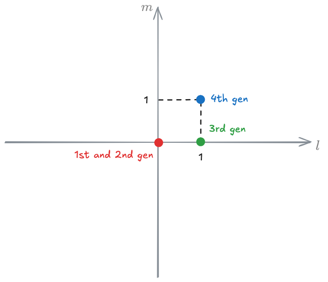
1st generation - GM model

In the 1st generation of the [[#General motors car-following models (1958-1961)]] the sensitivity $α$ is considered constant:
$\begin{aligned} {\ddot{x}}_{n + 1} (t + Δ t) & = α \cdot [{\dot{x}}_{n} (t) - {\dot{x}}_{n + 1} (t)] \\ [\frac{m}{s^{2}}] & = [\frac{1}{s}] \cdot [\frac{m}{s}] \end{aligned}$
The acceleration of the follower is directly proportional to the relative speed between the leader and the follower.

$α$ and $Δ t$ are considered constant parameters to calibrate.

When DM tried to calibrate the model, they realized that they weren't able to find a constant falue for $α$ . This was instead possible for $Δ t$ .

The sensitivity parameter showed large variability depending on the driving conditions, suggesting that maybe this parameter was not a constant.

2nd generation - GM model

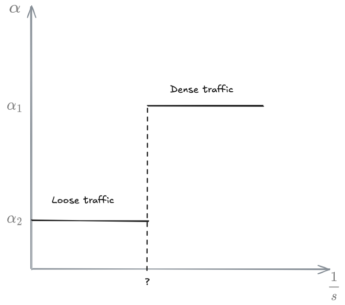
04 - Microscopic traffic flow modeling - OMT 2024-12-16 16.30.23.excalidraw.png
%%🖋 Edit in Excalidraw%%

GM observed that $α$ had too much variation. So, they decided to use 2 different values of $α$

3rd generation - GM model

Since they didn't know at what point you would get a new value of $α$ , GM decided to use a linear function to describe $α$ :

04 - Microscopic traffic flow modeling - OMT 2024-12-16 16.32.57.excalidraw.png
%%🖋 Edit in Excalidraw%%

${\ddot{x}}_{n + 1} (t + Δ t) = \frac{α_{0}}{[x_{n} (t) - x_{n + 1} (t)]} [{\dot{x}}_{n} (t) - {\dot{x}}_{n + 1} (t)]$
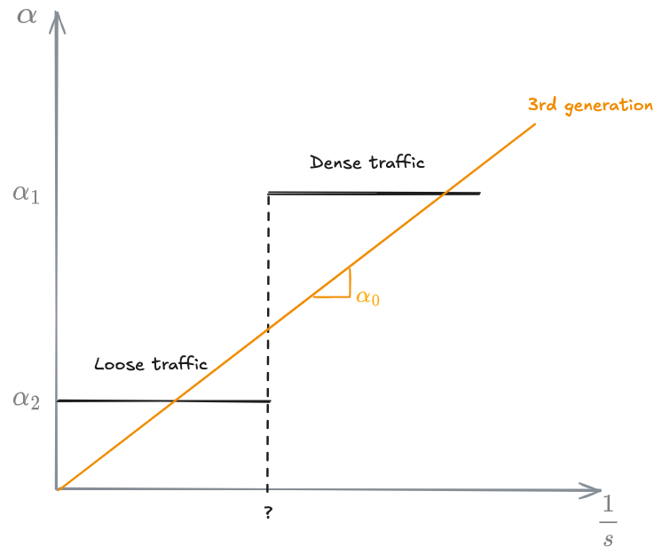
where $α_{0}$ is the sensitivity coefficient and is measured in $[\frac{m}{s}]$ .

So, $α_{0}$ is a speed. It gives the linkage between microscopic and macroscopic traffic flow models.

Relation between 3rd gen micro model and Greenberg macro model

Integrating the 3rd generation model in time, we get (notice that the relative speed is the derivative of the spacing):
${\dot{x}}_{n + 1} (t + Δ t) = α_{0} \ln (x_{n} (t) - x_{n + 1} (t)) + C$
In terms of speed:
$V = α_{0} \ln (\frac{C}{k})$
We can try to find the constant of integration $C$ by the following initial conditions:
$V = 0 k = k_{j}$
then:
$0 = α_{0} \ln (\frac{C}{k_{j}}) ⟹ C = k_{j}$
and we get:
$V = α_{0} \ln (\frac{k_{j}}{k})$
which looks exactly like the [[03 - Fundamentals of traffic flow modeling - OMT#Greenberg k-v model (1959)]] with $α_{0} = v_{0}$ , which is the optimal speed.

4th generation - GM model

In the 4th generation, they proposed that $α_{0}$ is not constant but dependent on the speed of the follower:
$α_{0} = α^{'} {\dot{x}}_{n + 1} (t)$
the model is then
${\ddot{x}}_{n + 1} (t + Δ t) = \frac{α^{'} {\dot{x}}_{n + 1} (t)}{[x_{n} (t) - x_{n + 1} (t)]} [{\dot{x}}_{n} (t) - {\dot{x}}_{n + 1} (t)]$
where

$α^{'}$ is a-dimensional

This means that how attentive you are, not only depends on the spacing, but also on the traveling speed (more attentive the faster you go)

! We still have 2 parameters.

5th generation - GM model

2 parameters are added, $n$ and $l$ . They have no known physical meaning, but they're useful to hav more flexibility in calibrating the model.

${\ddot{x}}_{n + 1} (t + Δ t) = \frac{α^{'} [{\dot{x}}_{n + 1} (t)]^{n}}{[x_{n} (t) - x_{n + 1} (t)]^{l}} [{\dot{x}}_{n} (t) - {\dot{x}}_{n + 1} (t)]$

All the [[#General motors car-following models (1958-1961)]] are a particular case of the 5th gen model.

04 - Microscopic traffic flow modeling - OMT 2024-12-16 16.49.33.excalidraw.png
%%🖋 Edit in Excalidraw%%

3 car following model

This is an extension of the [[#General Motors]] models, proposed by Fox-Lemann in 1967. They account for 3 cars at the same time, where the follower is affected both by the leader and the leader's leader stimuli:

{\ddot{x}}_{n + 2} (t + T) = α {\dot{x}}_{n + 2} (t + T) [ω_{1} \frac{{\dot{x}}_{n + 1} (t) - {\dot{x}}_{n + 2} (t)}{x_{n + 1} (t) - x_{n + 2} (t)} + ω_{2} \frac{{\dot{x}}_{n} (t) - {\dot{x}}_{n + 1} (t)}{x_{n} (t) - x_{n + 1} (t)}]

Collision avoidance models

collision avoidance models

The main principle behind collision avoidance models is that a driver will place themselves at a certain distance from the leading vehicle, such that in the event of an emergency stop by the leader, the follower will come to rest without striking the leading vehicle

Models that fall under this category are:

Pipes (1953)
Gipps (1981)
Mahut (1999-2001) - improvement over Gipps' model

Pipes model (1953)

Pipes car-following model (1953)

Pipes' was one of the first [[#Car following models]] ever proposed.

It comes from the [[California Driving Code]]. The code stated: "Drivers should leave a gap of one vehicle length for every $10 m p h$ of traveling speed."

This translates to:

pipes model (1953)

04 - Microscopic traffic flow modeling - OMT 2024-12-15 17.06.10.excalidraw.png

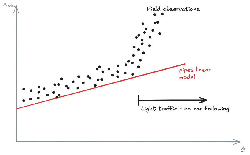
According to the Pipes model, Drivers should leave a gap of one vehicle length for every $10 m p h$ of traveling speed:
$s_{n + 1} (t) = l_{n + 1} + \frac{{\dot{x}}_{n + 1} (t)}{10 m p h} l_{n + 1}$

This model works quite well although:

For low speeds, it yields spacing considerably lower than the measured one
It only works for heavy traffic (this is true for any car following model)

This model is incredibly simple: in fact it has only 1 parameter: the follower length $l_{n + 1}$ .

Gipps model (1981)

The principle is to keep a safe distance from the leading vehicle to avoid crashing.

It's a time discrete model, meaning it needs time steps.

properties

According to Gipps, the model should have the following properties:

Model should mimic behaviour of real traffic
Parameters should have physical meaning on driver and vehicle (easy calibration)
Time step = reaction time

This model basically works as an optimization problem where the user wants to maximize their speed according to 2 constrains:

Acceleration constraint: each vehicle has a maximum acceleration it can be subject to
Safety constraint: the trajectory of each vehicle is affected by that of the vehicle in front

Gipps uses the following notation:

$τ :$ reaction time
$V_{n} :$ derived speed of vehicle $n$
$a_{n} :$ maximum acceleration with the driver of vehicle $n$ wishes to undertake
$b_{n} :$ most severe braking for vehicle $n$
$s_{n - 1} :$ effective length of vehicle $n - 1$
${\hat{b}}_{n - 1} :$ estimated most severe braking for vehicle $n - 1$ (empirically)

ACCELERATION:
The vehicle tries to reach desired speed.

v_{n} (t + τ) = v_{n} (t) + 2.5 a_{n} τ (1 - \frac{v_{n} (t)}{V_{n}}) (\sqrt{0.025 + \frac{v_{n} (t)}{V_{n}}})

SAFETY:

v_{n} (t + τ) = b_{n} τ + \sqrt{b_{n}^{2} τ^{2} - b_{n} [2 (x_{n - 1} (t)) - s_{n - 1} - x_{n} (t)]} \cdot \sqrt{- v_{n} (t) τ - \frac{v_{n - 1} (t)^{2}}{{\hat{b}}_{n - 1}}}

After estimating both quantities, Gipps selects the minimum value of speed between the two, and assigns that to the vehicle.

Computationally fast
Reproduces real macroscopic behaviour
Includes reaction time

Mahut

A generalization of [[#Gipps model (1981)]].

2 models:

constrained (linear)
unconstrained (non linear)

Drive is subject to maximum speed from 2 constraints:

Acceleration constraint
- Physical limitations for speed and acceleration
- Driver's desire for comfort
Safety constraint
- Affected by next downstream vehicle
- Related to steady state properties and condition of stability
Traffic stream is homogeneous
Free flow speed constant for each vehicle
State vector (position, speed, acceleration) denoted by $a (t)$

Mahut's model introduces stochastic variations over Gipps' model

Newell

[[Newel Notes_Catalina Vargas.pdf]]

Based on trajectories.

x_{n} (t + τ_{n}) = x_{n - 1} (t) - d_{n}

Trajectory of follower is the same as the leader with a translation in space and time.
2 parameters:

$τ_{n} :$ translation in time
$d_{n} :$ translation in space

Spacing is proportional to velocity

Doesn't consider reaction time directly but there is a variable, $T_{n}$ , that can be associated to it.

There is a relation with macroscopic behaviour.

Only on homogeneous highways
No lane change
Does not specify

Every driver has a desired speed. If the leader is going faster, the follower will just keep the desired speed.

Hidas (2005)

[[Hidass Lane changing model.pdf]]

Car following model has sudden deceleration
- If spacing goes below the desired spacing, it uses emergency breaking deceleration

Time to End of Lane. Lane is ending, lane change needs to happen.

The model is a dynamic process that keeps updating. It's described through a flow chart that goes through many different states and changes the behaviour of DVA accordingly.

Intelligent Driver Model

[[IDM.pdf]]

The Intelligent Driver Model was developed by Triber, Hennecke and Helbing around the year 2000.

Its high level goals are:

Simulate intelligent drivers - braking and accelerating
Microscopic, time and space continuous
1 lane behavior
1 or multiple types of vehicles

The general equation of the model takes the following form:

Acceleration = max acceleration \times (1 - freeflow acceleration - interaction term)

This is expressed as:

{\dot{v}}_{α} = a^{(α)} [1 - {(\frac{v_{α}}{v_{0}^{(α)}})}^{δ} - {(\frac{s_{α}^{*} (v_{α}, Δ v_{α})}{s_{α}})}^{2}]

where:

$v_{α} :$ current speed
$v_{0}^{(α)} :$ desired speed
$s_{α}^{*} :$ desired spacing (see expression later)
$s_{α} :$ current spacing

As the current speed approaches the desired speed, acceleration is reduced more and more.

s_{α}^{*} = s_{0}^{α} + s_{1}^{α} \sqrt{\frac{v_{α}}{v_{0}^{α}}} + T^{α} v + \frac{v Δ v}{2 \sqrt{a (α) b (α)}}

where:

$s_{0} :$ minimum distance between cars
$s_{1} :$ spacing dependent on speed
$a, b :$ comfortable acceleration and deceleration
$T :$ headway in time

Some parameters need calibration:

$a, b$
$T$
Some are easily defined:
$s_{0}, s_{1}$
$δ :$ acceleration exponent (usually =4)
$v_{0} :$ desired speed

The diagram above shows possible traffic states according to this model.

FT: Free Flow traffic
Most of these states appear after a perturbation (one driver performs hard braking)
Reproduces well many real world jams
Subject to histeresis: perturbances always make traffic worse
Heavy traffic may not cause congestion until a small perturbance appears without change in other conditions

Comments:

Many parameters but only a few affect the model
- Choice of $a$ , $b$ and $T$ is still not trivial and may cause instability
No reaction time (explicit). There is a safe headway as $T v$
Some states can only happen if drivers are "not intelligent"
There are some jams that happen despite the bad driving behaviour. This means that even self driving could not solve all traffic issues
Can't do simulation with infinite precision
- If we ever get inside safety margin, we would get negative speeds

Krauss

Krauss' model is the default model available in SUMO.

Krauss found some problems with the existing models:

Unknown ranges of application
How models relate to each other
These problems are mainly caused by:
Too many assumptions
Large number of parameters

It's a [[#Collision avoidance models]].

It introduces a randomization parameter.

Krauss presents a family of models based on Gipps's family:

High acceleration
High deceleration low acceleration
Low deceleration low acceleration
with the following considerations:
Discrete space coordinates
Deterministic jamming
Multilane Traffic
Computational performance

It has some pretty strong assumptions:

l = τ = 1

both spacing and reaction time are set equal to 1 (units are not specified). This is quite strong. A lot of information is lost in this. The accuracy of the model is still pretty good because of the randomization parameter, $η$ .

The random parameter is added as a random reduction in speed:

v (t + Δ t) = max (0, v_{d e s} (t) - η)

where

η \in Uniform (0, ε a)

where

ε \in [0, 1]

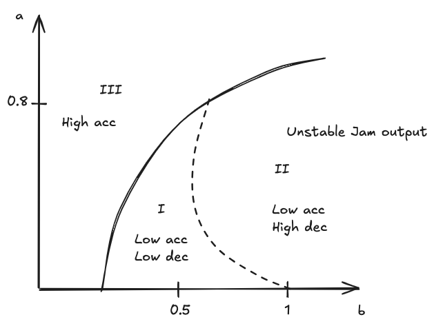
Depending on the values chosen for $a$ and $b$ , Krauss models can be classified into 3 types:

Type I:

Big jams
Stable output jam flow
Phase separation, metastability, capacity drop

Type II:

Some jamming
Unstable output jam flow
Phase separation not clear, jams don't scale

Type III:

No structural jamming
Homogeneous traffic