04 - Trip Distribution Modeling - TDBM

Trip Distribution is the second step in the modeling stage of the classic 4 stage framework.

In terms of an O/D matrix like the following, in this step we try to model each and every $d_{i j}$ :

\begin{matrix} d_{11} & d_{12} & \dots & d_{1 n} & P_{1} \\ d_{21} & d_{22} & \dots & d_{2 n} & P_{2} \\ ⋮ & ⋮ & d_{i j} & ⋮ & ⋮ \\ d_{n 1} & d_{n 2} & \dots & d_{n n} & P_{n} \\ A_{1} & A_{2} & \dots & A_{n} \end{matrix}

where:

$d_{i j} :$ number of trips from TAZ $i$ to TAZ $j$
$P_{i} :$ tot number of trips generated by TAZ $i$
- It's the sum of the colums
$A_{i} :$ tot number of trips attracted by TAZ $j$
- It's the sum of the rows
$n :$ tot number of TAZs

Along this note, the number of trips from TAZ $i$ to TAZ $j$ will sometime be indicated with the symbol $t_{i j}$

Introduction

Trip distribution models are conceptually simple but give a hard time when we try to integrate them with the other models in the 4 stage process (for example, often, the sum of the number of trips from one zone does not add app to the modelled marginal total).

assumptions

Production ( $P_{i}$ ) and attraction ( $A_{j}$ ) for each zone is known by purpose

Notation

Lower case letters indicate observations:

\begin{array}{r} t_{i j}, o_{i}, d_{j} \end{array}

trips, trips originated, trips attracted

Uppe rcase letters represent values we are trying to model:

$T_{i j}^{k n} :$ trips from $i$ to $j$ by mode $k$ and person type $n$ (population segment group)
$O_{i}, D_{j} :$ total number od trips originating at zone $i$ and attracted to zone $j$ , respectively

If a subscript or superscript is omitted, we are impying a summation over that index:

\begin{aligned} T_{i j}^{n} & = \sum_{k} T_{i j}^{k n} \\ T & = \sum_{i j} T_{i j} \\ t & = \sum_{i j} t_{i j} \end{aligned}

Key principles

Here we list some key principle of trip distribution models:

Bigger TAZs produce/attract more trips
Closer TAZs attract more trips
Further TAZs attract less trips: we will consider a deterrence function ( $f (c_{i j})$ where $c_{i j}$ is the cost from TAZ $i$ to $j$ ).

Trip distribution models

Demand origin-destination
- Beckmann & Golob: $t_{i j} = A_{i} B_{j} C_{i j}^{- γ} ⟹ t_{i j} = A_{i}^{α} B_{j}^{β} C_{i j}^{- γ}$
- Wardrop: $t_{i j} = \frac{P_{i} P_{j} e^{- θ D_{i j}}}{\sum_{k} P_{k} e^{- θ D_{i k}}}$
Choice
- Logit: $t_{i j} = G_{i} \frac{e^{- V_{i j}}}{\sum_{k} e^{- V_{i k}}}$
Opportunity
- Of intervention...
- Of competence...
#Gravity models
[[#Entropy models]]

Gravity models

Gravity models are #Trip distribution models inspired by [[Newton's law of gravitational attraction]]
the model for gravitational attraction between two masses.

basic trip distribution gravity model

The basic gravity model is:
$t_{i j} = k \frac{O_{i} D_{j}}{C_{i j}^{θ}}$
where:

$k :$ a constant
$O_{i} :$ all trips generated from zone $i$ (= to marginal total $P_{i}$ )
$D_{j} :$ all trips attracted to zone $j$ (= to marginal total $A_{j}$ )
$C_{i j} :$ generalized cost from zone $i$ to zone $j$
$θ :$ another parameter (if $θ = 2$ then we have exactly the same form of Newton's law)

Variations of this model exist:

{\begin{cases} t_{i j} = k O_{i} D_{j} e^{- θ C_{i j}} \\ t_{i j} = k O_{i}^{α} D_{j}^{β} C_{i j}^{- γ} Cobb-Douglas \\ t_{i j} = k O_{i}^{α} D_{j}^{β} e^{- θ C_{i j}} \end{cases}

As we can see, these models have several parameters that need to be calibrated. At first, this might look like a difficult task:

t_{i j} = k O_{i}^{α} D_{j}^{β} C_{i j}^{θ}

But, if we apply a logarithmic transformation on both sides, we can simply the calibration process:

\begin{aligned} \log (t_{i j}) & = \log (k O_{i}^{α} D_{j}^{β} C_{i j}^{θ}) = \\ = \log (k) + α \log (O_{i}) + β \log (D_{j}) + θ \log (C_{i j}) \end{aligned}

As we can see, this has now become a simple linear model in the form:

Y_{i j} = β_{1} + β_{2} X_{2} + β_{3} X_{3} + β_{4} X_{4}

that can be easily estimated as a linear regression model.

We considered $O_{i}, D_{j}, C_{i j}$ known and we have a sample for $t_{i j}$ . so we can find estimates for $\hat{α}, \hat{β}, \hat{γ}$ .

As anticipated before, the issue with these kind of models is that the sum of the estimated ${\hat{t}}_{i j}$ along $i$ or $j$ does not always give the marginal totals. What we expect is:

\begin{array}{r} O_{i} = \sum_{j} {\hat{t}}_{i j} \\ D_{j} = \sum_{i} {\hat{t}}_{i j} \end{array}

but this often does not happen. When this is the case singly or doubly constrained [[#Growth factors]] must be applied.

In order to predict future demand, growth factors are usually used

Growth factors

[[#Uniform growth factor]]
#Singly constrained growth factor
[[#Doubly constrained growth factor]]

Uniform growth factor

The uniform growth factor is a simple way to predict future trips. Given data for a base year, we simply apply a growth of a certain percentage to every O/D pair.

The following table shows the base year trips:

A growth factor of $20 %$ ( $f$ ) is applied. We calculate the future trips $T_{i j}$ from the base trips $t_{i j}$ as:

T_{i j} = f \cdot t_{i j}

Singly constrained growth factor

The Singly constrained growth factor is used when marginal totals of either production or attraction are not equal to the sum of the corresponding $t_{i j}$ .

The following examples assumes that there is a difference in the origin totals ( $O_{i}$ ).

The base OD matrix is shown:

Notice how $O_{i} = \sum_{j} t_{i j}$ difference from the theoretical marginal total (the target in the table). For example, for TAZ 1, the ration between target and estimated origins is $a_{1} = 1.13$ . Notice also how the ratio is different for each TAZ.

Let $a_{i}$ be the ratio for origin $i$ , then we apply the following transformation:

T_{i j} = a_{i} \cdot t_{i j}

and we get:

After the transformation we can see that $O_{i}$ is now always equal to the target.

observation

Since the $T_{i j}$ are expectations, they do not need to be integer numbers.

Doubly constrained growth factor - Biproportional Fitting (BPF)

The Doubly constrained growth factor is used when marginal totals of both production and attraction are not equal to the sum of the corresponding $t_{i j}$ .

This method is also known under the name: Bi-proportional fitting (BPF).

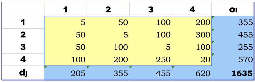
We start from the following base O/D matrix:

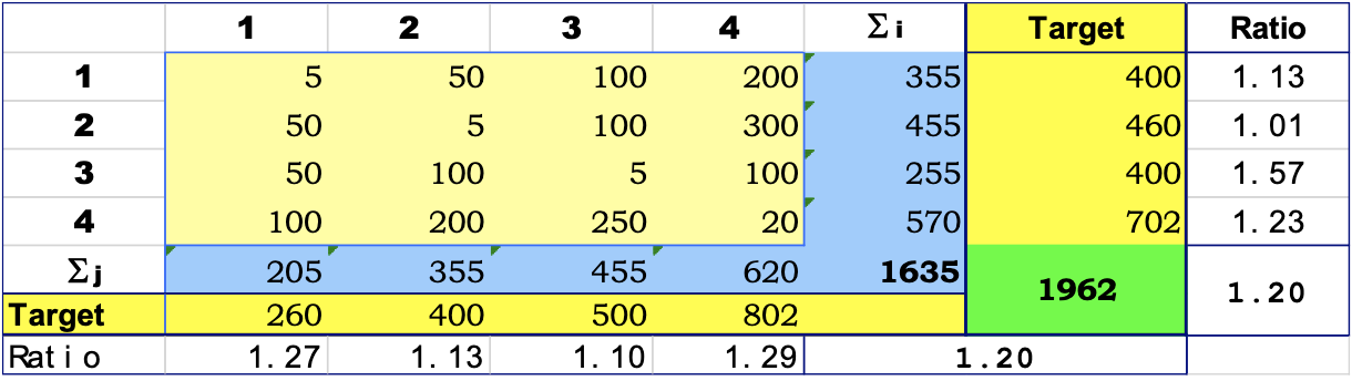
In this case there is not a direct method to obtain a single growth factor. The same process described in [[#Singly constrained growth factor]] is applied several time alternatively for Origins and destinations until we get acceptable ratios between the marginal totals and the targets.

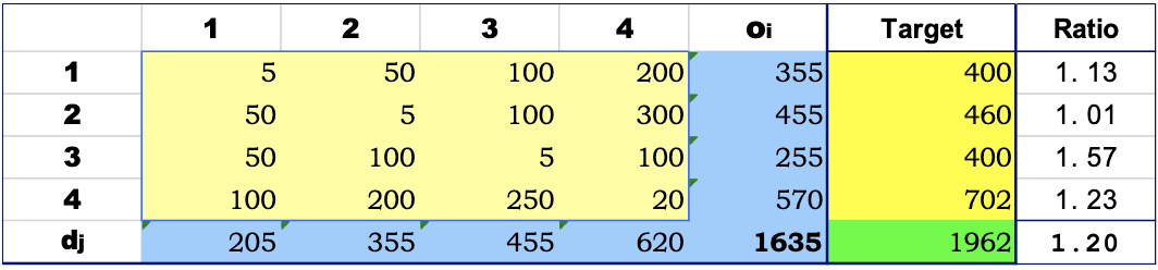
Calculate ratio for origins and apply it to every row
Calculate ratio for attractions and apply it to every column
Calculate ratio for origins and apply it to every row
Calculate ratio for attractions and apply it to every column
... And so on
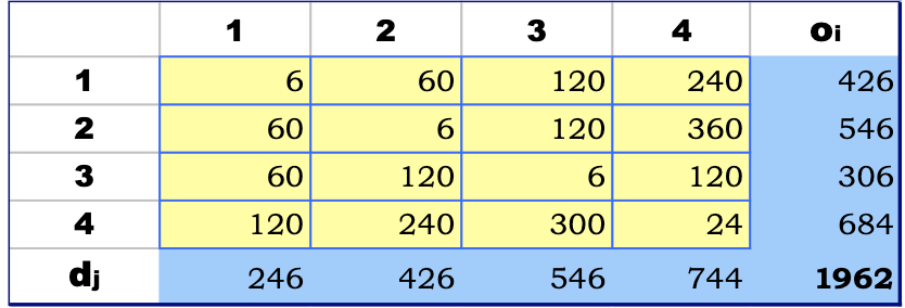
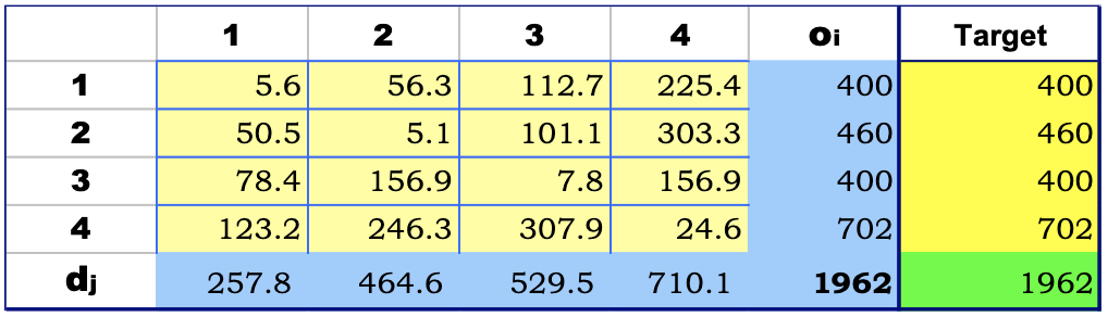
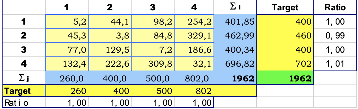
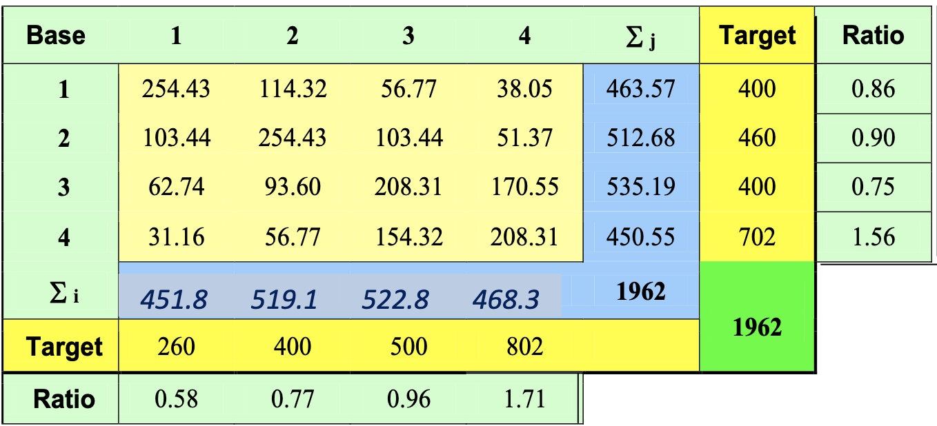
After not many iterations, we get a situation similar to that shown in the next table:

Limitations

Sparse matrices can cause problems when applying this method. If 0s are present, often the method will not converge. In this case, it is suggested to change these zeros to a low number of trips and try again.

Be careful though. It's important to distinguish between zeros by chance (sampling error) and structural zeros (there are some trips that cannot physically be made).

Synthetic distribution models

Synthetic distribution models are a kind of [[#Trip distribution models]] that generilize [[#Gravity models]] and try to bring more robust internal consistency. In their most general form:

T_{i j} = A_{i} O_{i} B_{j} D_{j} f (C_{i j})

where:

$A_{i}, B_{j} :$ balancing factors ensuring trip-end constraints are met (so to obtain internally consistent models)
$f (C_{i j}) :$ a functional for the travel cost between zone $i$ and zone $j$

Several functionals are proposed for the cost:

$f (C_{i j}) = e^{- β C_{i j}} :$ exponential function
$f (C_{i j}) = α C_{i j}^{- β} :$ power function
$f (C_{i j}) = α C_{i j}^{- β} e^{- γ C_{i j}} :$ combined function (gamma)
$f (C_{i j}) = α e^{- β \ln^{2} (C_{i j} + 1)} :$ lognormal function
$f (C_{i j}) = α e^{- β \ln^{2} (\frac{C_{i j}}{γ})} :$ top lognormal function

Notice how each of these functionals has one or more parameters that need to be calibrated. This is one of the main problems in applying this model.

Apply a synthetic distribution models

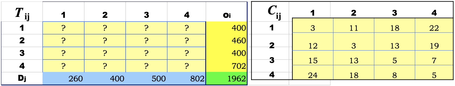
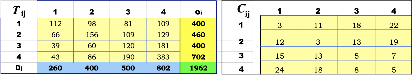
In this section we will see how to use #Synthetic distribution models to fill in the cells of an O/D matrix (calculate $T_{i j}$ ).

We will describe the process for a general functional $f (C_{i j})$ but keep in mind that the tables shown are using the functional $f (C_{i j}) = e^{- β C_{i j}}$ (for some value of $β$ ).

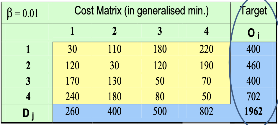
We start from a cost matrix. This matrix contains the cost $C_{i j}$ in the yellow cells. In the blue cells, the marginal totals $O_{i}$ and $D_{j}$ are shown.

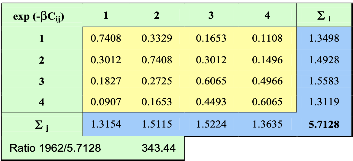
Now we apply the functional to the whole matrix: take any cell and calculate $f (C_{i j})$ . Whatch out, now the blue cells contain the sums of the yellow cells:

Now we need to apply the #Doubly constrained growth factor - Biproportional Fitting (BPF) method. To do so, we need a starting matrix containing trips. We can obtain it multiplying everything by an expansion factor calculated as:

f = \frac{\sum_{i} O_{i}}{\sum_{i} f (C_{i j})} \equiv \frac{\sum_{j} O_{j}}{\sum_{j} f (C_{i j})}

In this case, it would be:

f = 343.44 = \frac{1962}{5.7128}

Yielding:

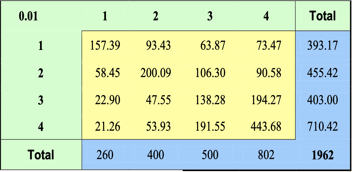
from this, the BPF method is applied and we get the following matrix (now every cell contains a value that represents the number of trips):

Entropy models

Entropy models are based on the law of entropy:

t_{i j} = A_{i} O_{i} B_{j} D_{j} e^{- k C_{i j}}

❗❗❗❗❗❗❗❗❗❗❗❗
❗❗❗ COMPLETARE ❗❗❗
❗❗❗❗❗❗❗❗❗❗❗❗

Hyman's method

When we #Apply a synthetic distribution models, we need to know the parameter of the cost functional $f (C_{i j})$ . In the case of

f (C_{i j}) = e^{- β C_{i j}}

we can use Hyman's method to find the appropriate value of $β$ .

To apply this method we need:

$o_{i} :$ observed trip production
$d_{j} :$ observed trip attraction
$C_{i j} :$ cost matrix
$M T L :$ Mean trip length
- This is a parameter that is calculated from a smaller sample

Assumptions:

$f (C_{i j}) = e^{- β C_{i j}} :$ $β$ unknown
OD matrix can be obtained through #Doubly constrained growth factor - Biproportional Fitting (BPF)

As for other sections in this note, example numbers are shown in tables.

Let's assume we start from the following condition:

We have marginal totals but no $t_{i j}$ and a cost matrix ( $C_{i j}$ ). We also have a Mean Travel Cost $M T L = 10^{'}$ (min).

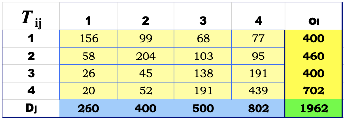
We have to start with some value of $β$ . We can set $β_{0} = 1$ . Then we calculate $β_{1}$ as:

β_{1} = \frac{1}{M T L} = 0.1

Now we have all the information needed to apply the #Synthetic distribution models. We get the following matrix:

Let's now check the value of Mean Travel Time that we get from this: $M T L_{1}$ . The Mean Travel Time is a weighted average of the travel costs using trips as weights. In this case:

M T L_{1} = \frac{156 * 3 + 99 * 11 + \dots + 58 * 12 + \dots}{156 + 99 + \dots + 58 + \dots} = 8.7

The expected value of MTL is 10. They are too different, we need another iteration

Now we set $β_{2}$ :

β_{2} = \frac{M T L_{1}}{M T L} β_{1} = 0.087

Calculate again the trip matrix as before and again $M T L_{2}$ . If the difference with $M T L$ is still too big, then keep going. For following iterations, set $β$ as:

β_{n} = \frac{(M T L - M T L_{n - 2}) β_{n - 1} - (M T L - M T L_{n - 1}) β_{n - 2}}{M T L_{n - 1} - M T L_{n - 2}}

For the example used so far we get:

β^{*} = 0.0586

Let $n$ be the iteration counter. The Hyman's method can be summarized in the following steps.
Let

M T L_{n} = \sum_{i j} \frac{T_{i j}^{(n} C_{i j}}{\sum_{i j} T_{i j}^{(n}}

$n = 0$

Set $β_{0} = 1$
Do nothing

$n = 1$

Set $β_{1} = \frac{β_{1}}{M T L}$
#Apply a synthetic distribution models
If $M T L_{1} \neq M T L$ go to next iteration, otherwise stop

$n = 2$

Set $β_{2} = β_{1} \frac{M T L_{1}}{M T L}$
#Apply a synthetic distribution models
If $M T L_{2} \neq M T L$ go to next iteration, otherwise stop

$n > 2$

Set $β_{n} = \frac{(M T L - M T L_{n - 2}) β_{n - 1} - (M T L - M T L_{n - 1}) β_{n - 2}}{M T L_{n - 1} - M T L_{n - 2}}$
#Apply a synthetic distribution models
If $M T L_{n} \neq M T L$ repeat, otherwise stop