02 - Dynamic Network Loading - TSM

[[03 - Fundamentals of traffic flow modeling - OMT#Macroscopic models]]

Dynamic Network Loading

• [?] In what way DNL goes from path flows to link flows?

With this method, we are trying to move from path flows to link flows.

We need to account for:

• [[#Link flow propagation models]]
• Node behaviour
• Lane-changing

Inputs and outputs - DNL

Inputs - DNL

• Network
• Time dependent short paths from each origin to each destination for each time interval
• O/D matrices
• Time dependent path flows

Outputs - DNL

• Link cost for each interval

• [?] Isn't the output the simulation? The trajectories of the vehicles?

Link flow propagation models

These can be classified in several ways. The most popular classificaiton is the division in macro, micro and meso -scopic models.

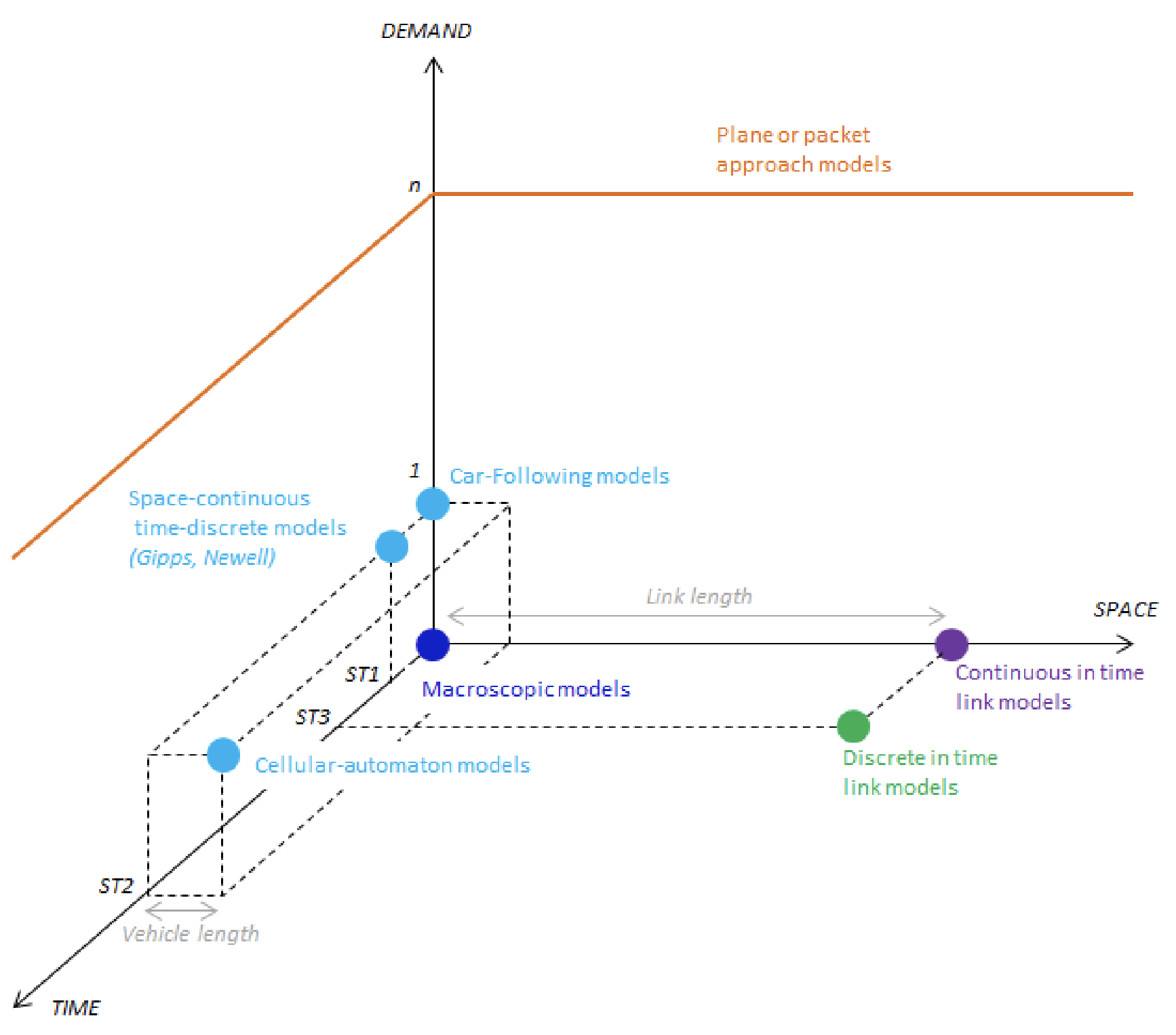
An alternative classification is that proposed by [[Astarita]] (2002), that can be summarised in the following diagram:

The diagram actually shows an adaptation of the classification proposed by Astarita.

In this classification, each model is classified based on the way the 3 core elements are treated:

• Demand
• Time
• Space

The closer to the origin, the more the variable is considered as continuous. The farther we go, the greater discretisation we have.

According to Astarita, these are some models we can have:

• Microsimulation models
• Continuous in time models
• Discrete in time link models
• Models following a packet approach
• Macroscopic simulation models

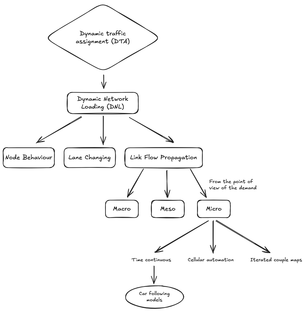
From the point of view of the demand, we only have:

• Macroscopic models
• Mesoscopic models
• Microscopic models

Here, we are mainly interested in microscopic models:

Microscopic traffic flow models

They model the actions (such as accelerations and lane changes) each driver takes as a response to the surrounding environment. They are especially suited to study heterogeneous traffic streams (different kinds of vehicles). With these models we can distinguish different kinds of drivers and vehicles.

In theory, the results from a microscopic models should, when aggregated, give the same results as a corresponding macroscopic model. In practice, this is not usually the case.

What's needed in microscopic models

• Acceleration strategies - vehicles should try to approach the free flow speed
• Braking strategies - vehicles should be able to brake to avoid colliding with obstacles
• Safe distance - Vehicles should always maintain a safe distance from other vehicles

We typically assume that humans react to stimulus from other vehicles, with main influence caused by the leading vehicle.

The main parameter that characterises an individual is the reaction time.

Classification of microscopic simulation models

The following classification can be summarised in the diagram below:

Time-continuous models

These models are formulated as ordinary differential equations.

They consider:

• continuous time
• continuous space
• discrete demand (1 by 1)

They are mostly Car following models:

• GHR (General Motors)
• Safety distance or collision avoidance
• Linear
• Psychophysical
• Fuzzy
• IDM
• Desired spacing models

Cellular automation

Cellular automation models use integer variables to describe the dynamic state of the system.

• discrete time
• discrete space
  Time is discretised. Links are divided into cells which can be either occupied by a vehicle or empty.

Iterated coupled maps

Iterated coupled maps models fall in between #Time-continuous models and #Cellular automation models.

• discrete time
• continuous space
  The update time is considered as an explicit model parameter rather than an auxiliary parameter needed for numerical integration

Some examples are:

• Gipps
• Newell