Parsimonious models for Public transport network design
Parsimonious models for Public transport network design
Parsimonious models carry various advantages:
- [p] They have few assumptions and analytically tractable --> they provide a close solution
- [p] Low data requirements
- [p] Low computational complexity
- [p] Better system representation
- [p] Greater transparency
- [p] Higher sharpness or insight
for these reasons they are often used to analyse large transportation systems and can be physically realistic and accurate
They rely on a #Continuous approximation method:
Continuous approximation method
This method allows for the development of #Parsimonious models.
It consists in solving an optimisation problem in which we try to minimise the total cost defined as:
where:
is the length of the line
Finding the minimum means to derivate the function and set it equal to zero:
1D line
We will start by considering a 1 dimensional system with the following characteristics:
line length distance travelled by a generic user demand, uniformly distributed along the line length vehicle cruising speed vehicle constant acceleration/deceleration boarding and alighting time per passenger walking speed
Decision variables:
stop spacing (distance between stops) vehicles headway (time distance between 2 consecutive vehicles)
We need to find the total cost of travelling along the line. We have to distinguish:
User cost
The user cost can be decomposed in 3 components, relating to time:
From that we will calculate the #User Generalised Cost, as:
where:
value of time trip fare
User travel time
Access time
The Access time is the time it take the passenger to get from their origin to the closest bus stop (or from the stop to the destination).
Imagine we have a stretch of line like in the diagram:

Ignoring the transversal distance between the start of the jurney and the closest stop (which cannot be influenced by changing the decision variable), we are interested in the distance that a passenger has to travel to reach the closest stop.
This distance could have any value between
Considering the worst case, in which every user has to walk at least
Waiting time
The waiting time is the time a generic passenger has to wait at a bus stop before the bus arrives.
The extreme cases are:
- The bus arrives exactly at the same time as the user, then the waiting time is
- The bus leaves exactly as the user arrives, than they have to wait for the next bus:
The average waiting time is:
In Vehicle Travel time
The in vehicle travel time is the time that the generic passenger spends in the vehicle for their trip. It accounts for dwell times and acceleration. It can be divided in 3 components:
- Time spent travelling at constant speed
- Time spent accelerating and decelerating
- Time spent for passengers boarding and alighting
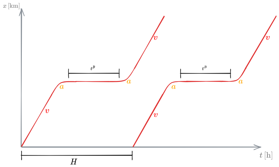
To evaluate these, it's useful to keep in mind a generic trajectory for a bus stopping at a bus stop:

1 - Time spent travelling at constant speed
If the user travels for a distance
This slightly overestimates the actual time. This way in fact we are also considering the space where the vehicle is not travelling at constant speed.
- [?] This slightly overestimates the actual time. This way in fact we are also considering the space where the vehicle is not travelling at constant speed
2 - Time spent accelerating and decelerating
Along the distance travelled, we have
At each stop, the time spent accelerating is
At each stop, the time spent decelerating is
- [?] Shouldn't the acceleration time, according to uniformly accelerated motion, be
. Why are we using ? ⏫
Then, the time spent not travelling at constant speed at each stop is
3 - Time spent for passengers boarding and alighting
Lastly, we need to account for the dwell time.
In order to calculate this, we need to know how many passengers will board at each bus stop.
- If the general demand per hour is
, then, along the whole corridor, the number of passengers boarding each vehicle will be ; - We only have to account for the proportion of travellers along the stretch of length
. Therefore, we will need to multiply the demand per bus by ; - For one pax, the dwell time is
Then, for the whole trip, the time spent stopping for boarding operations is:
IVTT:
We can now write the In Vehicle Travel Time as the sum of the aforementioned components:
User Generalised Cost
The user generalised cost is given by:
where:
value of time trip fare
that we can write explicitly as:
Time perception
The calculations done in the previous sections does not account for the fact that users perceive time differently depending on what they're doing. Therefore, when calculating the #User Generalised Cost we should account for this factor. The following table shows average and ranges values for time perception at different phases of the trip:

Operator costs
The operator costs include mainly these components:
- #Corridor length - V - Distance travelled by the fleet per hour (#Operation)
- M - #Fleet size (number of vehicles) and Work force per hour
After having calculated every one of the mentioned components, we can calculate the generalised operator cost:
where:
unitary cost of infrastructure per km and hour unitary cost based on distance travelled by fleet per hour unitary cost for fleet acquisition and crew operation
Corridor length
The corridor length is simply a constant:
We do not consider 2L as we are assuming a circular line. Then, the same infrastructure is used in both directions
Operation
The operation is caused by the distance travelled by the whole fleet per hour.
If the total length of the line is
Fleet size
The fleet size is given by the total amount of vehicles. In order to get this, we need the time spent by one vehicle to travel the whole corridor and divide it by the headway. The time spent by one vehicle is given by the corridor length over the #Commercial speed.
Commercial speed
The commercial speed is the average speed of a vehicle in a transportation line, accounting for each slow down.
It's given by the total distance in the corridor over the time spent in the corridor (the #In Vehicle Travel time calculated for a trip length of
where
1D line optimisation problem
The problem to solve is then:
subject to:
where
is the transfer time Maximum vehicle occupancy during peak hour vehicle capacity
2D line
A similar problem to the #1D line can be defined for a 2D line, where transfers between lines are possible.
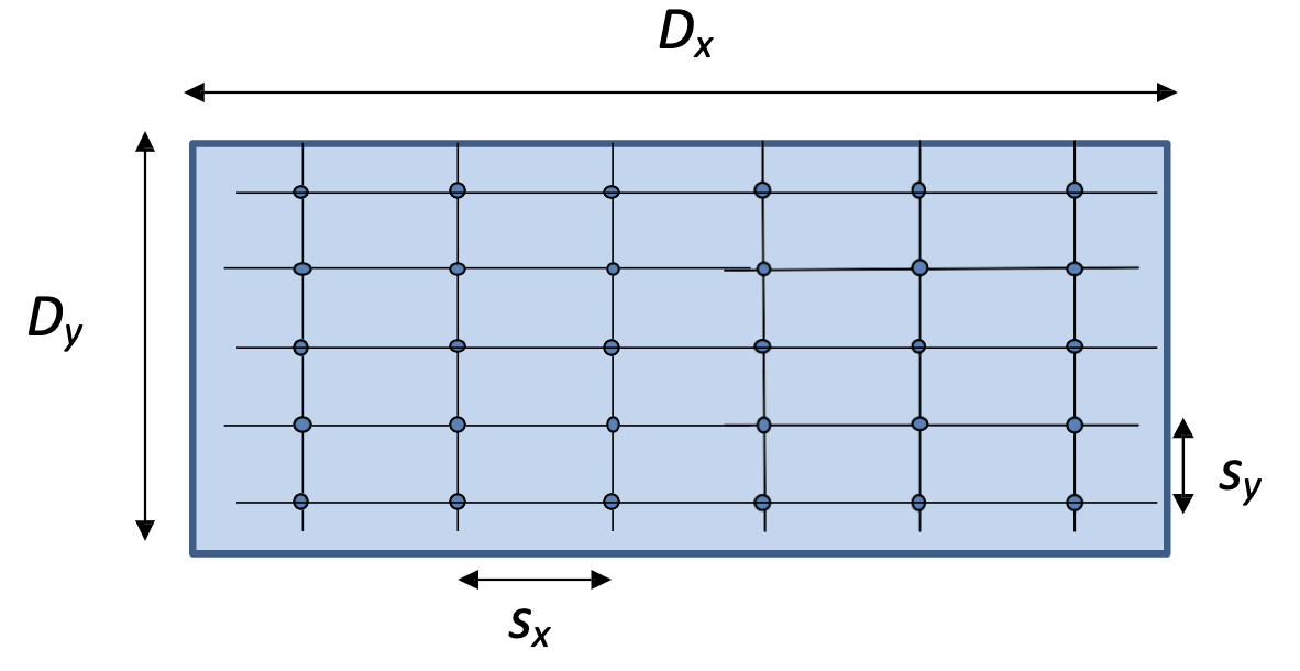
The easiest example is a grid system:
