04 - Microscopic traffic flow modeling - OMT
04 - Microscopic traffic flow modeling - OMT
Introduction
Microscopic traffic flow modeling falls under the scope of [[Car following theory]].
This kind of theories work well only for heavy traffic conditions.
Definitions
2 vehicles follow each-other.
The vehicle in front is referred to as Leader and is vehicle
Some parameters:
length of the vehicles The gap between the follower and the leader The spacing of the follower vehicle
Introduction
The objective of microscopic traffic flow modeling is trying to predict the trajectories of individual vehicles on space and time. The movement has 2 components:
- Longitudinal - Moving along the axis of the road
- Lateral - ie Lane changes
In this chapter we will only look at longitudinal models.
Spacing in central for 2 concepts:
- Traffic safety
- Infrastructure capacity
Safety vs flow
Spacing needs to ensure that drivers can react and adapt to new speeds of vehicles in front without colliding. In terms of safety, the larger the spacing, the safer. In contrast, a large spacing, at equivalent speed, causes a reduction in capacity of the infrastructure:
In terms of capacity, it would be ideal to have high speed and small spacing.
On the road, spacing is left to the driver perception of risk. It's the drivers that evaluates and decides what is the appropriate trade-off for each situation to guarantee safety. In other kind of transportations, like trains, it's the infrastructure that tells the driver the spacing, or better, it forces the appropriate spacing.
Automated driving
Automated driving promises to brake the trade-off [[#Safety vs flow]].
Autonomous vehicles can achieve very short reaction times. If we assume that all vehicles are able to communicate with each other, then the reaction time is barely the time it takes the information to travel from one veh to the other. The order of magnitude is
Therefore, Autonomous vehicles should be able to travel with very little spacing.
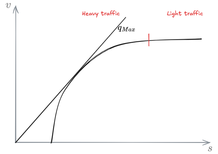
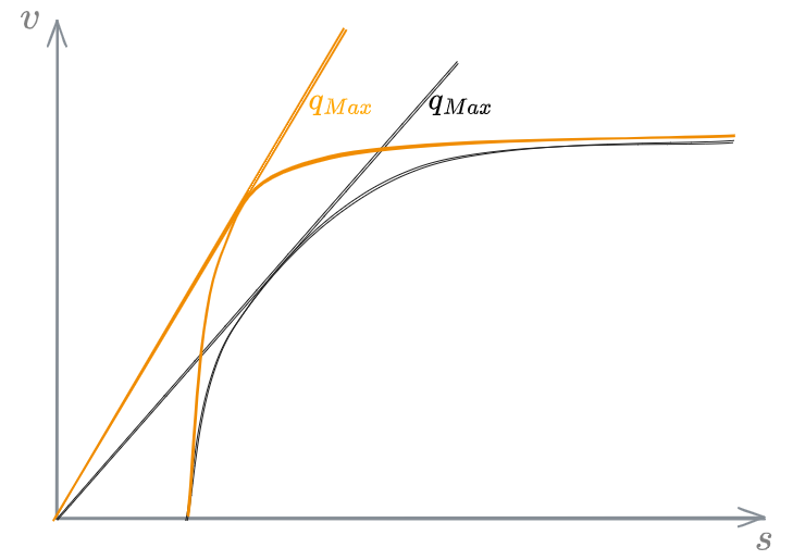
The diagram shown in [[#Safety vs flow]], with autonomous vehicles, could become more similar to the following:
Notice how the spacing will be fairly constant, despite the speed, in heavy traffic, to a point where spacing is not dependent on speed anymore in light traffic.
Platooning
What [[#Automated driving]] is supposed to achieve is known as platooning.
Platooning is a condition where many vehicles travel as if they were one, connected as a train.
Car following models
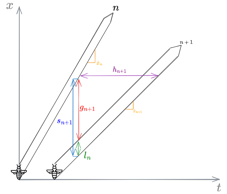
Several microscopic models were proposed during the years. Here we will see some of them. In order to study them, it's important to first understand the following graph:
From now on we will have to account for the vehicles length, hence, each vehicle is represented by a pair of trajectories (one for the front and one for the tail of each vehicle). All the main parameters are shown in the graph:
headway gap vehicle length spacing vehicles speed
The following relations can be deduced:
Now we are ready to see several models. Specifically, we will see:
- [[#Pipes car-following model (1953)]]
- [[#Forbes car-following model (1958)]]
- #General motors car-following models (1958-1961)
Pipes car-following model (1953)
Pipes' was one of the first [[#Car following models]] ever proposed.
It comes from the [[California Driving Code]]. The code stated: "Drivers should leave a gap of one vehicle length for every
This translates to:
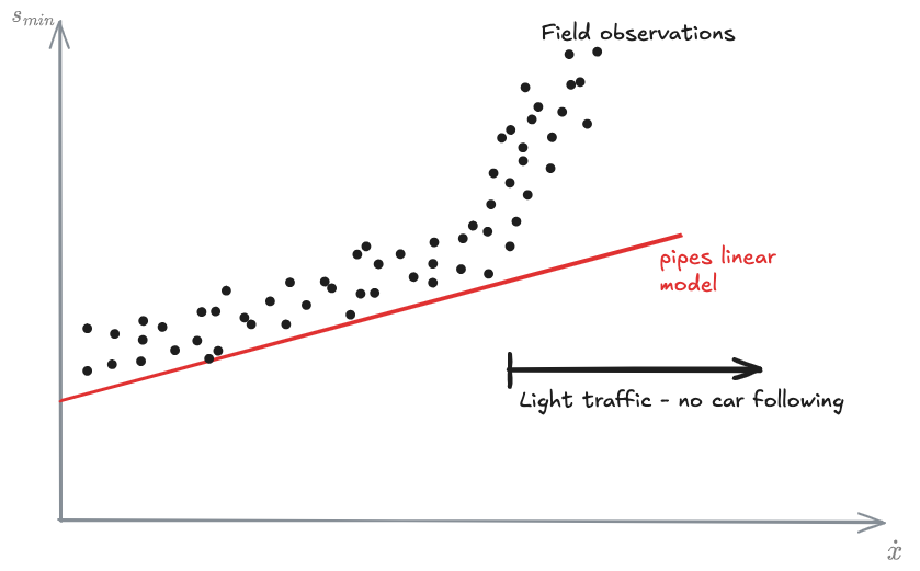
According to the Pipes model, Drivers should leave a gap of one vehicle length for every
This model works quite well although:
- For low speeds, it yields spacing considerably lower than the measured one
- It only works for heavy traffic (this is true for any car following model)
This model is incredibly simple: in fact it has only 1 parameter: the follower length
Forbes car-following model (1958)
In 1958, Forbes introduced [[Reaction time (traffic)]]
It was proposed that, in order to avoid collisions, the time gap between 2 vehicles should be at least equal to the reaction time.
Therefore, the headway should be the reaction time
Since the spacing is given by
Forbes model, formulated in terms of spacing, then becomes:
Like pipes' model, this is also linear. This time though, it is dependent on a parameter that is not fixed, meaning the model can be calibrated to better describe the specific traffic observed.
General motors car-following models (1958-1961)
In the late 50's, American company [[General Motors]] started developing some [[#Car following models]]
They developed several generations of a model. The models were calibrated using real world data.
General Motors car-following models fall under the spectrum of [[stimulus-response model]].
GM car following models
Stimulus-response models, in car-following theory, describe the acceleration of the follower as a function of the speed relative to the leader.
Response
In longitudinal movement, the follower can only react in 2 ways to what the vehicle in front does:
- Accelerate
- Decelerate
The response is therefore measured in terms of follower acceleration:
Stimulus
Sensitivity
measures how attentive you are to traffic.
- Response: follower acceleration -
- measured at a time (a reaction time after ) - If the stimulus happens at , the response always happens after the stimulus - Stimulus: Relative speed -
- Sensitivity: a proportionality factor (or function) -
The general model is always in the form:
Depending on the model generation then,
GM model Generations
1st generation - GM model
In the 1st generation of the #General motors car-following models (1958-1961) the sensitivity
The acceleration of the follower is directly proportional to the relative speed between the leader and the follower.
When DM tried to calibrate the model, they realized that they weren't able to find a constant falue for
The sensitivity parameter showed large variability depending on the driving conditions, suggesting that maybe this parameter was not a constant.
2nd generation - GM model
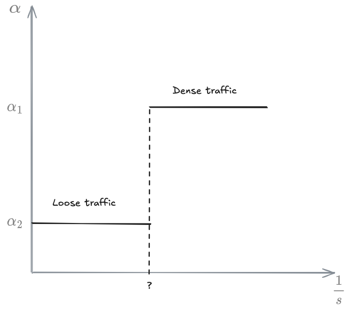
GM observed that
3rd generation - GM model
Since they didn't know at what point you would get a new value of
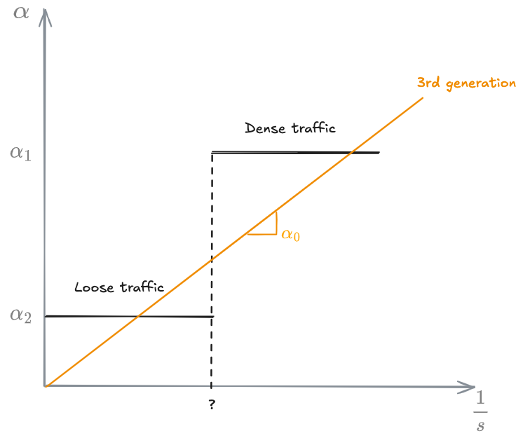
where
So,
Relation between 3rd gen micro model and Greenberg macro model
Integrating the 3rd generation model in time, we get (notice that the relative speed is the derivative of the spacing):
In terms of speed:
We can try to find the constant of integration
then:
and we get:
which looks exactly like the 03 - Fundamentals of traffic flow modeling - OMT#Greenberg k-v model (1959) with
4th generation - GM model
In the 4th generation, they proposed that
the model is then
where
is a-dimensional
This means that how attentive you are, not only depends on the spacing, but also on the traveling speed (more attentive the faster you go)
! We still have 2 parameters.
5th generation - GM model
2 parameters are added,
All the [[#General motors car-following models (1958-1961)]] are a particular case of the 5th gen model.
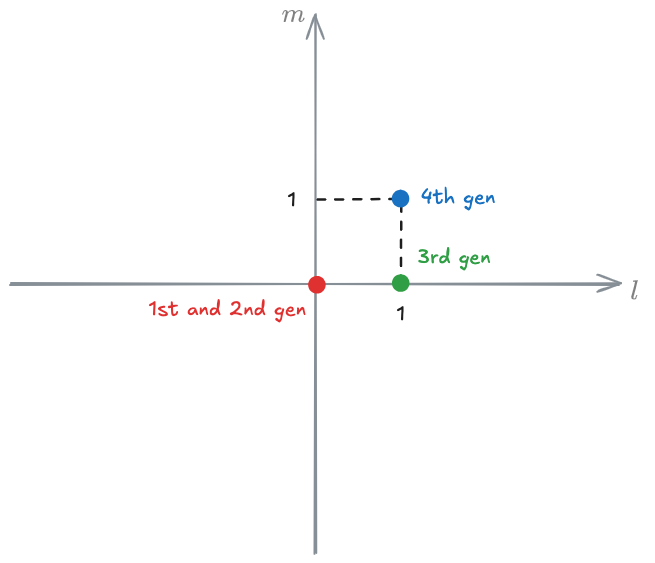
Traffic stability
The kind of equations we setup in the [[#General motors car-following models (1958-1961)]] define an oscillatory movement.
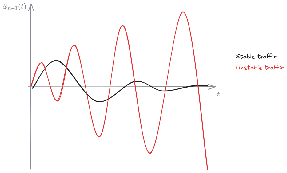
We can look at an instability parameter, found from the models:
Notice that
It can be shown that traffic is stable if:
If
This condition is valid for asymptotic stability: it's not only a pair of veh, it's a long queue of vehicles.

