03 - Fundamentals of traffic flow modeling - OMT

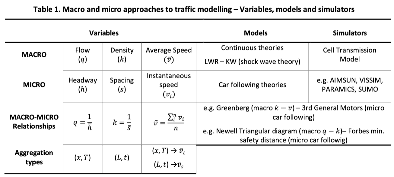
In traffic flow modeling, we can distinguish between

Macroscopic models
Microscopic models

In this chapter we will focus on #LWR Traffic flow theory.

Macroscopic models

macroscopic models

Macroscopic models predict the evolution in time of the macroscopic variables:

Flow - $q$
Density - $k$
Average Speed - $v$

They are very robust: it's difficult for things to go wrong in calculation. They only use a few parameters (3).

They are known with many different names:

Lightwill, Witham, Rehand (LWR) model
Continuous Traffic Flow Model
Shock-Wave theory
Cinematic Wave Theory

And are solved by some simulators - Calculation can be done by hand

Cell Transmission Model

Microscopic models

microscopic models

Microscopic models try to predict how one vehicle, the follower, follows another vehicle, the leader

Given the trajectory of the leader, we are interested in obtaining the trajectory of the follower.

They are very detailed, but use many many parameters (in the order of $10^{1}$ ).

In microscopic models, we work with microscopic variables:

Headway - $h$
Spacing - $s$
Instantaneous speed - $v_{i}$

Microscopic models are known as:

Car following theories

And are solve by computer simulators:

[[AIMSUM]]
[[VISSIM]]
[[PARAMICS]]
[[SUMO]] - which is [[Open Source]]

LWR Traffic flow theory

LWR theory postulates

LWR theory is based on 2 postulates:

postulates of lwr theory

#Conservation of vehicles
#Equation of state

Conservation of vehicles

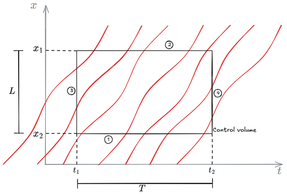
Given a control volume (space x time), the number of vehicles that enter the volume and that exit the volume must be equal.

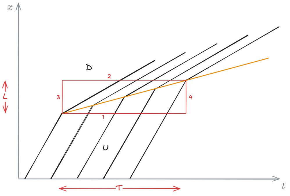
Look at the trajectories in the following diagram:

%%🖋 Edit in Excalidraw%%

!!! The control volume is just a mathematical object. From now on we will refer to control area. The control area is the physical space that we are observing (for example, a stretch of road).

Let

$m_{i} :$ Number of veh entering/exiting the control area
$n_{i} :$ Number of veh already in the control area
Then

m_{1} + n_{3} = m_{2} + n_{4}

The members can be rearrange to write:

m_{2} - m_{1} = n_{3} - n_{4}

We can express the conservation of vehicles principle as follows:

The difference between vehicles entering and exiting the control volume must be equal to the variation in storage in the control volume.

The last equation can be divided by the area of the control region in the graph:

\begin{aligned} \frac{m_{2} - m_{1}}{(t_{2} - t_{1}) (x_{2} - x_{1})} & = \frac{n_{3} - n_{4}}{(t_{2} - t_{1}) (x_{2} - x_{1})} \\ \frac{m_{2} - m_{1}}{T} \frac{1}{x_{2} - x_{1}} & = \frac{n_{3} - n_{4}}{L} \frac{1}{t_{2} - t_{1}} \\ (q_{2} - q_{1}) \frac{1}{x_{2} - x_{1}} & = (k_{3} - k_{4}) \frac{1}{t_{2} - t_{1}} \\ \frac{q_{2} - q_{1}}{x_{2} - x_{1}} & = \frac{k_{3} - k_{4}}{t_{2} - t_{1}} \\ \frac{Δ q}{Δ x} & = - \frac{Δ k}{Δ t} \end{aligned}

where at one point we have substituted the definitions of flow and density. Finally, at limit, the equation can be written as:

\frac{\partial q}{\partial x} = - \frac{\partial k}{\partial t}

conservation of vehciles principle

The difference between vehicles entering and exiting the control volume must be equal to the variation in storage in the control volume.
$\frac{\partial q}{\partial x} = - \frac{\partial k}{\partial t}$

Relative flow

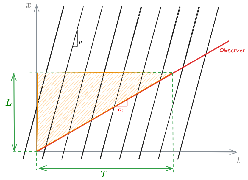
Let's consider the following time-space diagram:

%%🖋 Edit in Excalidraw%%

There are several vehicles traveling at speed $v$ and 1 observer traveling at speed $v_{0}$ .

The [[#Conservation of vehicles]] applies for any control volume we consider. Therefore, it applies for the one indicated in orange in the graph.

Given that:

$k :$ density of the vehicles traveling at speed $v$
$T :$ Time span considered
$L :$ Space considered

then, we have that:

{\begin{cases} k L = Number of vehicles entering from the left \\ q T = Number of vehicles exiting from the top \\ q_{0} T = Number of vehicles enetring from the bottom \end{cases}

where $q_{0}$ is known as the relative flow. This is the flow seen by the observer. According to the [[#Conservation of vehicles]]:

k L + q_{0} T = q T

So:

\begin{aligned} q_{0} T & = q T - k L \\ q_{0} & = q - k \frac{L}{T} \\ q_{0} & = q - k v_{0} \end{aligned}

according to the fundamental equation of trafic ( $q = k v$ ):

q_{0} = k (\underset{v_{r e}}{\underset{⏟}{v - v_{0}}})

where $v_{r e}$ is the relative speed between the observer and the the other vehicles.

relative flow

The relative flow, defined as
$q_{0} = k (v - v_{0})$
describes the amount of overtakes an observer experiences.

{\begin{cases} v_{r e} = 0 ⟹ No overtakes \\ v_{r e} > 0 ⟹ Traffic moves faster than the observer \\ v_{r e} < 0 ⟹ Traffic moves slower than. theobserver \end{cases}

In case $v_{0} < 0$ , then $q_{0} > q$ .

Equation of state

The second postulate of the [[#LWR Traffic flow theory]] is the existence of an equation of state. This means that the state of the system can be univocally determined applying one equation to a state variable.

In the fundamental equation of traffic, we can write one state variable as a function of the other 2. To get to the required equation of state, we need to go down to 1 degree of freedom. We need 1 extra equation.

This relation will be obtained empirically, meaning it is a regression of some measurement.

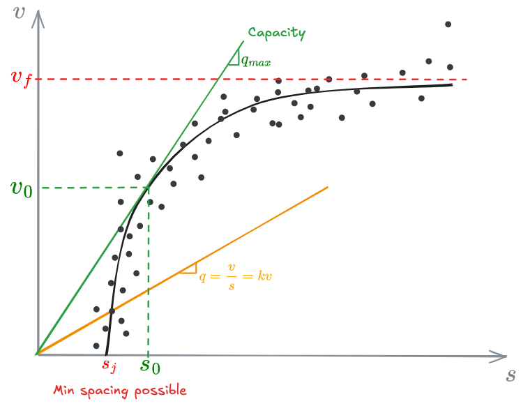
Let's imagine taking data points of speed against spacing:

%%🖋 Edit in Excalidraw%%

The graph shows the empirical relation between average speed and spacing. Notice that as spacing increases, also velocity increases until speed starts to approach a constant value, $v_{f}$ , known as free-flow speed.

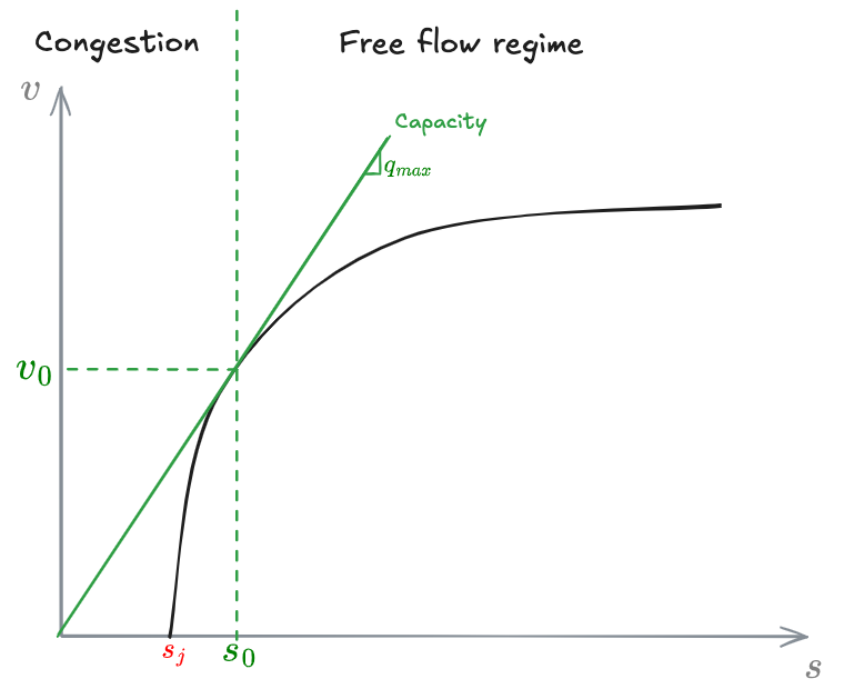
Remembering the fundamental equation of traffic flow, $q = k v = \frac{v}{s}$ , we can see that, for each point on the curve, the slope of the line passing through that point and the origin gives the flow in that state.

From this it's fairly easy to find the maximum flow, known as capacity of the infrastructure, as the tangent line.

From the state diagram, we can also define some new concepts:

[[#Congestion regime]]
[[#Traffic regime]]

Congestion regime

%%🖋 Edit in Excalidraw%%

Free-flow regime

free flow traffic

We have free flow traffic when we work on spacings (density) grater (less) than those relative to the capacity.

Congestion

congestion

We have congestion when we work on spacings (density) less (greater) than those relative to the capacity.

Traffic regime

Light traffic

light traffic

We have light traffic when the speed is not dependent on the spacing or density

Heavy traffic

heavy traffic

We have heavy traffic when the speed is dependent on the spacing or density

Density speed models

The first model was proposed by [[Bruce Greenshield]]. It's known as [[#Greenshield k-v model]]. We will see the following models:

[[#Greenshield k-v model]]
[[#Greenberg k-v model (1959)]]
[[#Underwood k-v model (1961)]]
[[#Edie k-v model]]

Greenshield k-v model

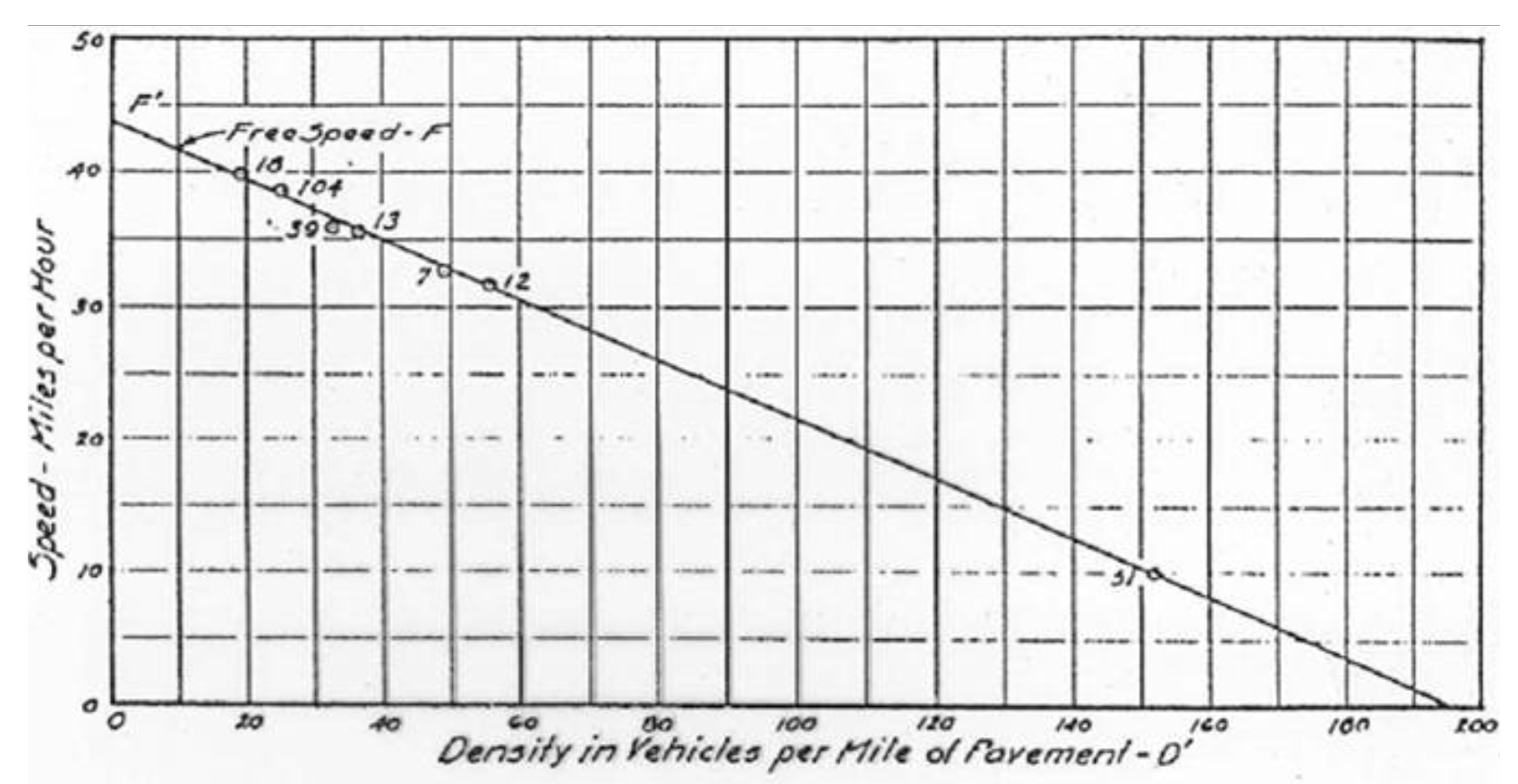
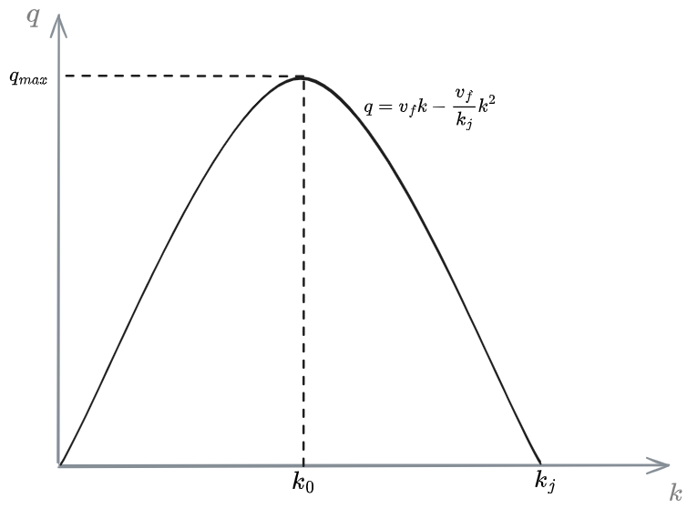
The figure above shows the original Greenshield k-v model. He described the average speed as a function of density, requaring 2 calibration parameters

the greenshield $k-v$ model

Greenshield k-v model - 03 - Fundamentals of traffic flow modeling - OMT 2024-12-06 17.18.32.excalidraw.png

$v = v_{f} (1 - \frac{k}{k_{j}})$
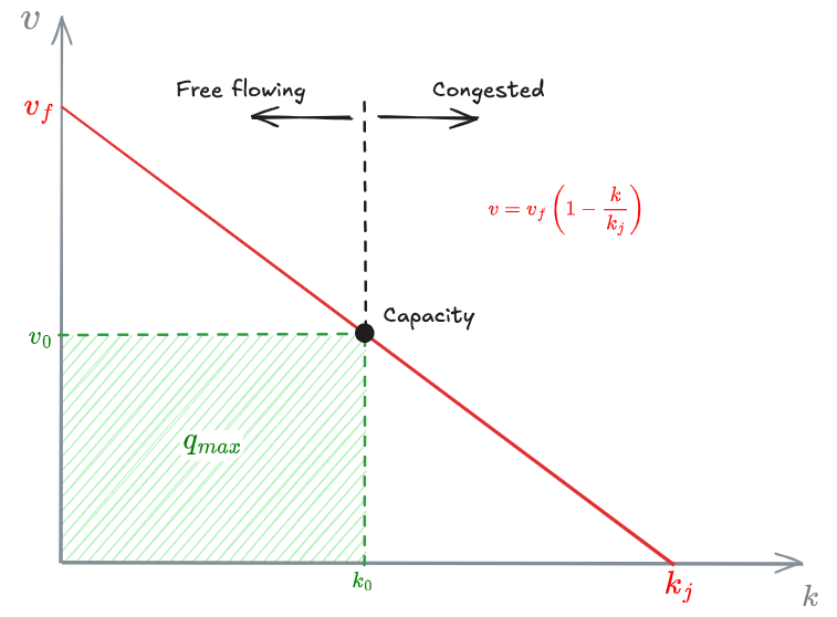
where:

$v_{f} :$ Free flow speed - Speed at which vehicles travel when density is very low
$k_{j} :$ Jam density - Maximum density at the infrastructure when vehicles are in a gridlock jam, completely stopped

Given $q_{m a x}$ is the maximum flow of the infrastructure, the capacity, this is given by the area of the rectangle of sides $v_{0}$ and $k_{0}$ .

The capacity point also distinguishes between two states:

Congestion
Free flowing

finding $q_{max}$

$v_{0}$ and $k_{0}$ can be obtained as follows. According to the fundamental equation of traffic and to the Greenshield model
${\begin{cases} q = v k \\ v = v_{f} (1 - \frac{k}{k_{j}}) \end{cases}$
Combining the 2 equations:
$\begin{aligned} q & = v_{f} (1 - \frac{k}{k_{j}}) k = \\ = v_{f} k - \frac{v_{f}}{k_{j}} k^{2} \end{aligned}$
To find the maximum of this funciton, we can derive and impose equal to 0:
$\begin{aligned} \frac{\partial q}{\partial k} = \frac{\partial}{\partial k} (v_{f} k - \frac{v_{f}}{k_{j}} k^{2}) & \overset{!}{=} 0 \\ v_{f} - 2 \frac{v_{f}}{k_{j}} k & = 0 \\ k = \frac{1}{2} k_{j} \end{aligned}$
So,
$k_{0} = \frac{1}{2} k_{j} v_{0} = \frac{1}{2} v_{f}$

03 - Fundamentals of traffic flow modeling - OMT 2024-12-06 17.31.49.excalidraw.png

Greenberg k-v model (1959)

Greenberg, in 1959, proposed a model that works very well in the congested part of the diagram, but not so much in the free flow.

greenberg $k-v$ model

Greenberg k-v model - 03 - Fundamentals of traffic flow modeling - OMT 2024-12-06 17.35.46.excalidraw.png

$v = v_{0} \ln (\frac{k_{j}}{k})$

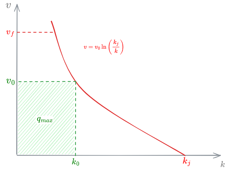
Since, mathematically, this model has velocity appriximating infinity for very low values of $k$ , the model is usually cut at the free flow speed, $v_{f}$ .

Underwood k-v model (1961)

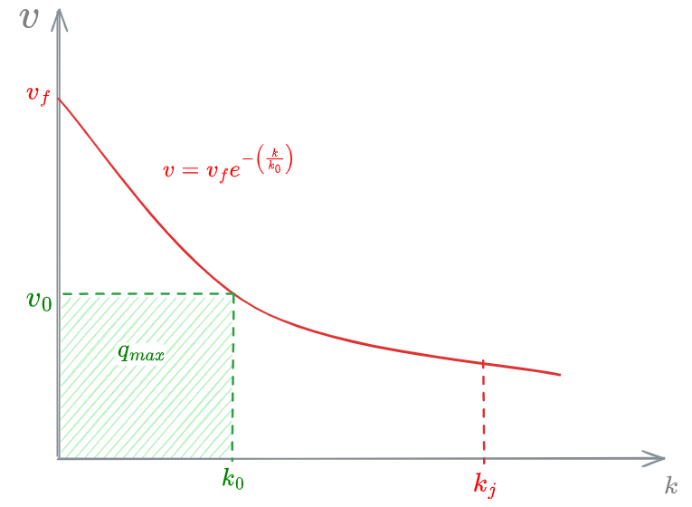
Underwood, in 1961, proposed a model calibrated for free flow condition, but that doesn't work well in congestion

underwood $k-v$ model

Underwood k-v model - 03 - Fundamentals of traffic flow modeling - OMT 2024-12-06 17.41.25.excalidraw.png

$v = v_{f} e^{- (\frac{k}{k_{0}})}$

Edie k-v model

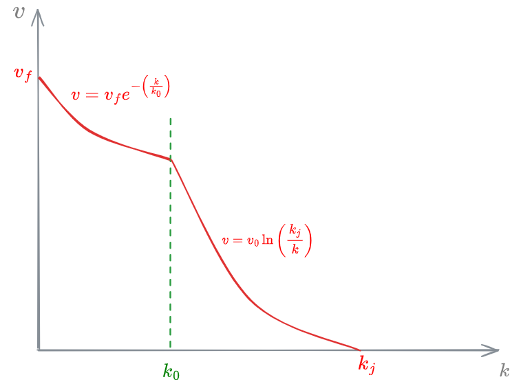
Edie, in 1961, decided to merge the [[#Greenberg k-v model (1959)]] and [[#Underwood k-v model (1961)]] in order to obtain one unique model that would work well for both free flow traffic and for congestion. This is simply the merging of the 2 functions cutoff at the capacity point $k_{0}$ .

edie $k-v$ model

Edie k-v model - 03 - Fundamentals of traffic flow modeling - OMT 2024-12-06 17.45.41.excalidraw.png

Traffic shock-wave

traffic shock-wave

Whenever there is a change in the state of traffic, such as an acceleration or deceleration, the information of such change travels in traffic. The travel of information is referred to as a traffic shock-wave. This means that in different points in space and time, the change in traffic state happens only once the shock-wave reaches that point.

Traffic shockwave speed

Look at the trajectory diagram below. There are several vehicles travelling at speed $v_{1}$ that then start to move at speed $v_{2} < v_{1}$ .

%%🖋 Edit in Excalidraw%%

Let's apply the [[#Conservation of vehicles]] to the red square:

\begin{aligned} m_{1} + n_{3} & = m_{2} + n_{4} \\ \underset{State U}{\underset{⏟}{m_{1} - n_{4}}} & = \underset{State D}{\underset{⏟}{m_{2} - n_{3}}} \end{aligned}

Let $q_{U}$ and $q_{D}$ be the flows for states $U$ and $D$ respectively. Similarly for $k_{U}$ and $k_{D}$ for densities. Then, the following relations stand:

\begin{aligned} m_{1} & = q_{U} T & n_{4} & = k_{U} L \\ m_{2} & = q_{D} T & n_{3} & = k_{D} L \end{aligned}

So we get:

q_{U} T - k_{U} L = q_{D} T - k_{D} L

Dividing both members by $T$ , defining $\frac{L}{T} = u$ :

q_{U} - k_{U} u = q_{D} - k_{U} u

from which we find:

u = \frac{q_{U} - q_{D}}{k_{U} - k_{D}} = \frac{Δ q}{Δ k}

that is defined as the shockwave speed.

traffic shockwave speed

The speed of a traffic shock-wave between 2 stationary traffic states is determined by the increase in flow over the increase in density:
$u = \frac{Δ q}{Δ k}$
If:

$u > 0 :$ wave travles in same direction of traffic
$u < 0 :$ wave travles in opposite direction of traffic

Fundamental diagram of traffic

The fundamental diagram of traffic is a density-flow diagram ( $k - q$ ). It's vastly used because a lot of information can be derived from it by simple inspection.

The typical shape of a fundamental diagram of traffic is the following:

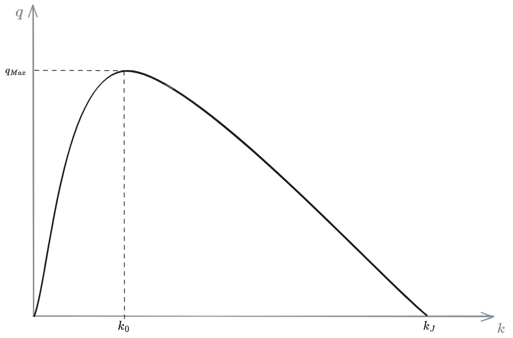
Traffic will be on any point of that curve and each point resembles a different traffic state.

A TRAFFIC STATE ON THE GRAPH

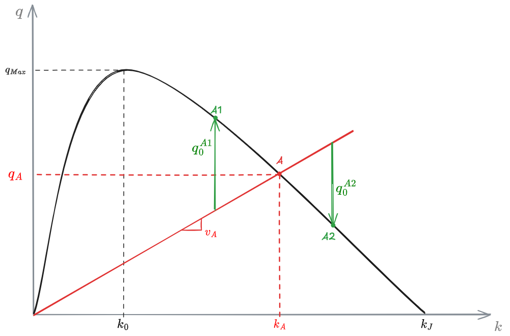
Look at traffic state A.

$k_{A}$ is the density in state $A$
$q_{A}$ is the flow in state $A$
By definition, the speed can be found as $\frac{q}{k}$ . So:

v_{A} = \frac{q_{A}}{k_{A}}

This can be represented graphically by a line going through the origin and intersecting the diagram in point $A$ .

RELATIVE FLOW

From the same graph we can also obtain the #Relative flow
between an observer traveling at speed $v_{A}$ and any other traffic state. Here we can see the relative flow with A1, $q_{0}^{A 1} > 0$ and with A2, $q_{0}^{A 2} < 0$ .

FREE FLOW AND CAPACITY

Let's look at some specific states on the fundamental diagram (FD):

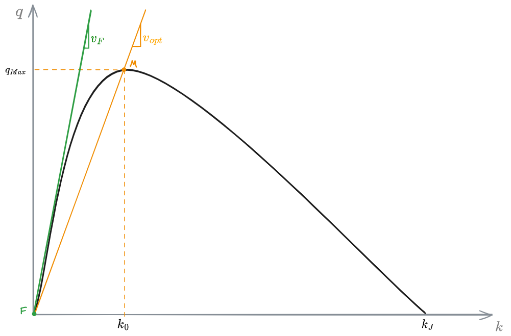
In the graph above 2 states are represented:

Maximum flow - State M
Free flow - State F

From the graph it's easy to gain the free-flow speed, $v_{F}$ and the optimal speed, $v_{o p t}$ .

SHOCK-WAVE SPEED

Let's now imagine traffic moves from state A to state B. It would be, in this case, an acceleration.

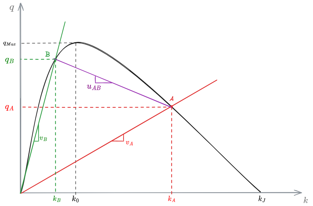
By definition, $u = \frac{Δ q}{Δ k}$ is the #Traffic shockwave speed between state A and state B. In the graph this can be read as the slope of the line going through A and B:

u_{A B} = \frac{q_{A} - q_{B}}{k_{A} - k_{B}}

Shocks and waves

The concept behind [[#LWR Traffic flow theory]] is that every change in traffic state causes a wave to be generated. If we're able to track the waves in space and time, we are then able to predict traffic evolution.

Just 2 situations are possible with traffic:

#Acceleration - LWR
#Deceleration - LWR

Acceleration - LWR

To study the acceleration transition, we will suppose a 1 lane road in which some vehicles are piled up behind a slow moving truck until time $t_{1}$ . At $t_{1}$ , the truck exits the road and vehicles behind it start accelerating. During the acceleration, the vehicles will travel at all the intermidiate speeds between the truck speed, $v_{B}$ and the free-flow speed, $v_{H}$ .

At every differential speed change a #Traffic shock-wave is generated.

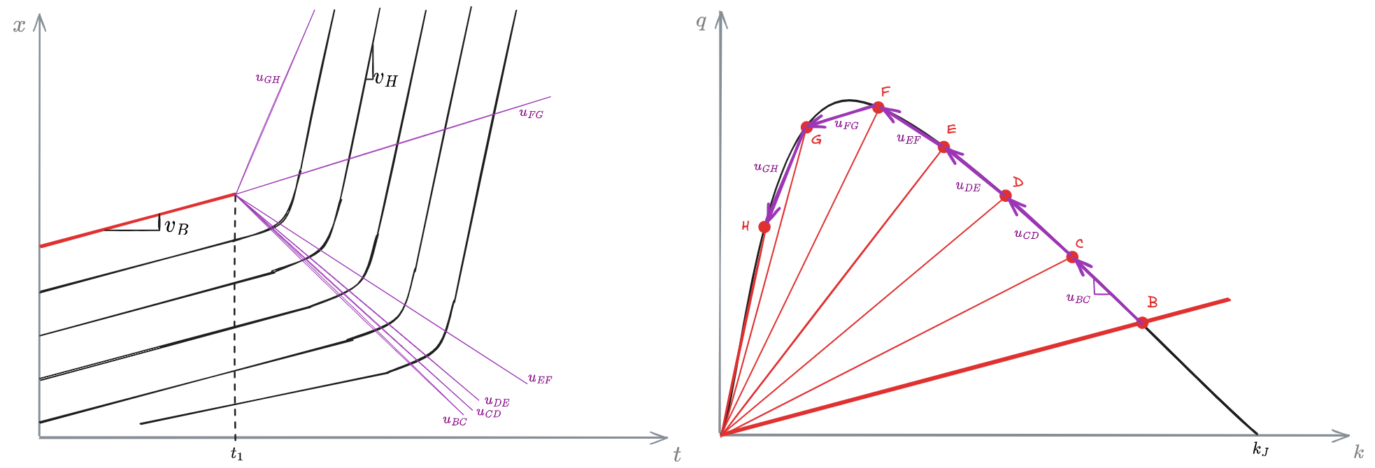
Each wave on the $t - x$ graph, with slope $u_{i j}$ , describes the threshold between traffic state $i$ and traffic state $j$ . Meaning we can predict the trajectory knowing the supposed slope from the $k - q$ #Fundamental diagram of traffic.

Notice that since each step is theoretically differential, there are infinitely many shockwaves every time we go from one state to another.

Deceleration - LWR

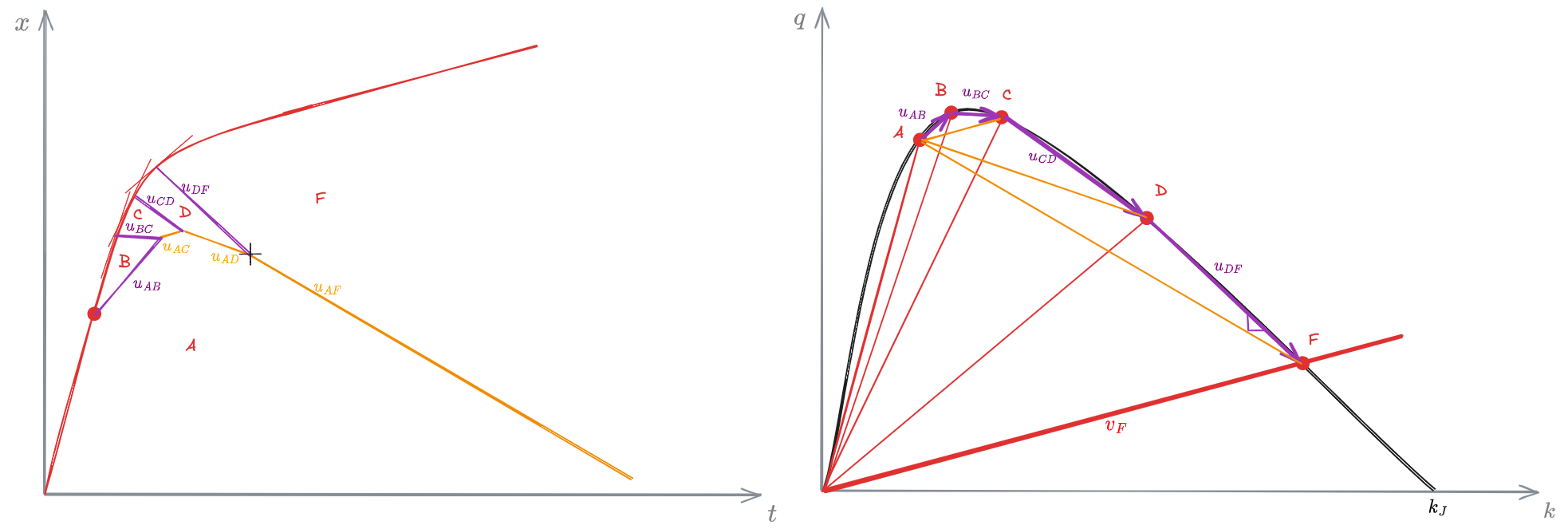
Now we just suppose that, on a stretch of road, vehicles are decelerating from speed $v_{A}$ to a lower speed $v_{F}$ , therefore moving from state A to state F. Differently from the #Acceleration - LWR, here waves do not tend to fan out. Instead, they tend to collide with one another.

When 2 waves collide, it means that 2 very different traffic states are colliding without any smooth transition. This generates yet an other wave, known as shock.

We will observe that initially there will be a smooth transition between state A and state F. Eventually though, only a single shockwave will remain changing abruptly from state A to state F.

Thinking of this in real life, when traffic slows down on a road, initially, the first cars have time to slow down gradually as the very first cause of the slowdown. As more cars arrive, the new ones will have less and less time to react until a point where one car is moving at free-flow speed until it finds the end of the queue that just formed.

LWR simplifications

From the explanation of #Shocks and waves it's clear that applying the model is not easy due to the infinitely many waves that generate between 2 states.

There are some simplifications that we can introduce to make things a lot easier. Specifically, we will add 2 assumptions:

Instantaneous accelerations/decelerations - LWR

We will consider every change in speed instantaneous. This means that, for each state change, only one #Traffic shock-wave is generated. This is particularly useful in #Deceleration - LWR, where infinitely many waves otherwise collide generating infinitely many shocks.

This assumption is actually quite justified when thinking that usually speed transition happen on a short time-span compared to the whole trajectory of a vehicle.

With this simplification, the graphs shown in #Deceleration - LWR will appear as the following:

This simplification still doesn't help much in accelerations, for which we need a new assumption: #Triangular fundamental diagram.

Triangular fundamental diagram

In the 1990 it was proposed to adopt a triangular #Fundamental diagram of traffic. This served 2 porpuses:

It was shown to actually be more accurate in describing present traffic, except for the area near capacity where the real data showed a smother transition
It made every state change in the two areas (#Congestion and #Free-flow regime) have the same #Traffic shockwave speed.

Now, the new state change, for #Acceleration - LWR, would look more like this

Now, in terms of waves, the state change $B \to H$ and $B \to C$ are equivalent. Therefore, the wave speed between for state change $B \to H$ is $w$ .

LWR Theory example

LWR theory limitations

All vehicles are considered equal
- Avg behavior (no overtakes, all at same speed)
Doesn't work well for light traffic
Can't give much precision - all results should be approximated
- $q - k$ graph comes from regression
- We are considering changes from happening instantaneously --> waves should be considered to be thick lines
Theory is not always stable
- In congested traffic speeds often fluctuate (stop and go), which is not predicted by this model