03 - Utility Demand function and Pricing - DME

%%
[[2024-11-08]]
%%

assumption - consumer economically rational

In the following discussion, we will assume the costumer to be economically rational:

The costumer will always try to maximize:

Consumption
Utililazation

Utility function

Let $X$ be the set of goods that an economy can produce:

X = {x_{1}, x_{2}, . . ., x_{n}}

For simplicity, in this chapter we will work with only 2 goods:

X = {x_{1}, x_{2}}

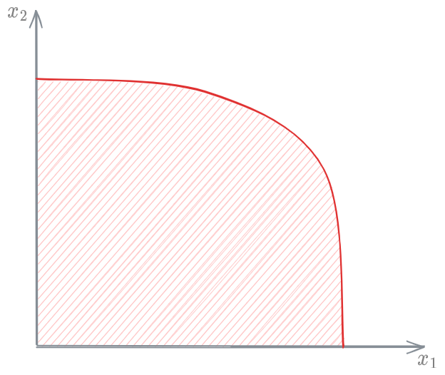
We can visualize this in the following graph:

%%🖋 Edit in Excalidraw%%

The area under the graph is the set of all possible combination of $x_{1}$ and $x_{2}$ .

The utility function is defined as follows:

utility function ($u$)

The utility function, is a function $u$ :
$u : R^{2} \to R$
such that $\forall (x_{1}, x_{2}), (y_{1}, y_{2}) \in X$ , if $(x_{1}, x_{2})$ is chosen over $(y_{1}, y_{2})$ , then $u (x 1, x_{2}) > u (y_{1}, y_{2})$ .

It's a particular function. We are not as much interested in the absolute value of the function as much as we are in the relative value. We don't really care how much $u (x_{1}, x_{2})$ or $u (y_{1}, y_{2})$ are, but more if $u (x_{1}, x_{2}) > u (y_{1}, y_{2})$ .

Properties of the utility function

The #Utility function is continuous

The #Utility function is monotonically increasing on every single variable:

\frac{\partial u}{\partial x_{i}} \geq 0 \forall i

The second derivative exists and is always negative or equal to 0 (the function is cuasi-convex):

\frac{\partial^{2} u}{\partial x_{i}^{2}} \leq 0 \forall i

The #Utility function, calculated in the empty set (in $(0, 0)$ ) is equal to 0:

u (0, 0) = 0

Types of utility function

Cobb-Douglas utility function

%%🖋 Edit in Excalidraw%%

The Cobb-Douglas utility function has the following value:

u (x_{1}, x_{2}) = x_{1}^{a} x_{2}^{b}

where

$a, b :$ are positive coefficients that measure the consumer preferences.

Quasilinear utility function

%%🖋 Edit in Excalidraw%%

The Quasilinear utility function has the following expression:

u (x_{1}, x_{2}) = ν (x_{1}) + x_{2}

where:

$ν (x_{1}) = \sqrt{x_{1}}$ or $ν (x_{1}) = \ln (x_{2})$

Linear utility function

The linear #Utility function is works well for [[#Perfectly substitutive goods]]:

u (x_{1}, x_{2}) = a x_{1} + b x_{2}

where:

$a, b > 0$

Other utility function

The other #Utility function works well for [[#Perfectly complementary goods]].

u (x_{1}, x_{2}) = min {a x_{1}, b x_{2}}

where:

$a, b > 0$

Indifference curve

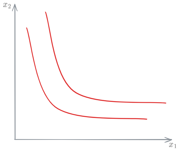
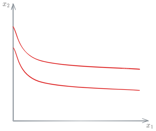
indifference curve

The indifference curve is the locus of points $(x_{1}, x_{2})$ where the #Utility function remains equal

Budget constrain

Let

$m :$ the total budget available
$p_{1}, p_{2} :$ Respectively the unit prices of goods 1 and 2
Then

p_{1} x_{1} + p_{2} x_{2} \leq m

%%
[[2024-11-13]]
%%

Theory of election

,
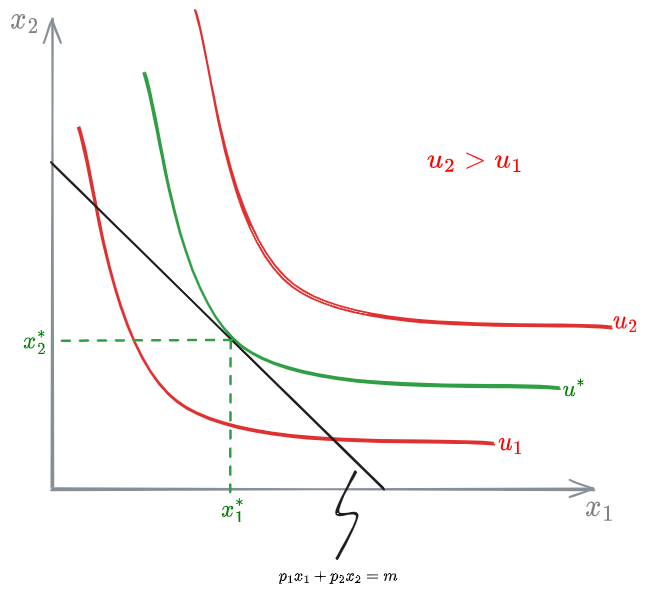
What combination $(x_{1}, x_{2})$ will the consumer choose?

Reminding that the consumer is rational, we have an optimization problem:

max_{(x_{1}, x_{2})} u (x_{1}, x_{2})

subject to:

p_{1} x_{1} + p_{2} x_{2} \leq m

%%🖋 Edit in Excalidraw%%

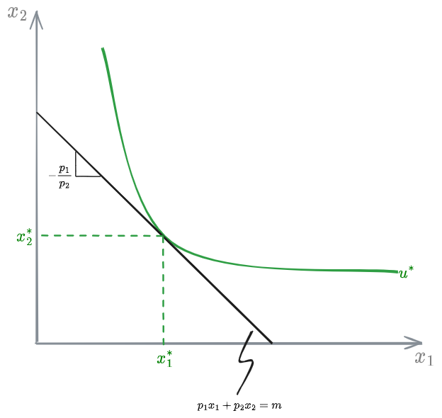
The solution to the problem is given by the utility such that the iso-utility curve is tangent to the constraint, in the tangent point:

(x_{1}^{*}, x_{2}^{*})

Relation of Marginal Substitution

%%🖋 Edit in Excalidraw%%

teorema

In order to maintain the [[#Utility function]] constant, the ratio between the production of good 1 and good 2 needs to be equal to the Relation of Marginal Substitution:
$R M S = - \frac{p_{1}}{p_{2}}$

Proof:
Keeping $u (x_{1}, x_{2})$ constant can be written as forcing its Differential equal to 0:
$\begin{aligned} d u & \overset{!}{=} 0 \\ d u & = \frac{\partial u}{\partial x_{1}} d x_{1} + \frac{\partial u}{\partial x_{2}} d x_{2} \overset{!}{=} 0 \end{aligned}$
From this we can write:
$\frac{d x_{1}}{d x_{2}} = - \frac{\frac{\partial u}{\partial x_{2}}}{\frac{\partial u}{\partial x_{1}}} \overset{△}{=} R M S$
Notice that, in the optimum point, the ratio $\frac{d x_{1}}{d x_{2}}$ must be equal to the slope of the budget $- \frac{p_{1}}{p_{2}}$
q.e.d.

Particular cases

Perfectly substitutive goods

perfectly substitutive goods

Two goods are perfectly substitutive when the consumer is willing to substitute one goods for an other with no change with a 1:1 ratio:

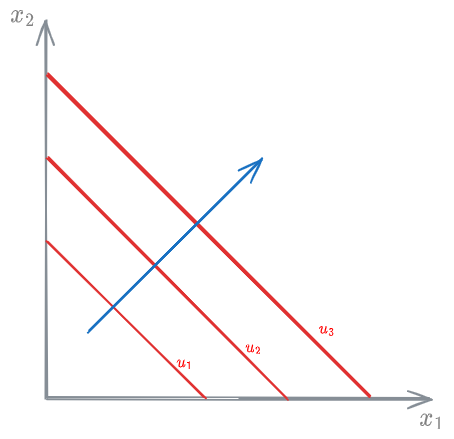
Perfectly substitutive goods - 03 - Utility Demand function and Pricing - DME 2024-12-01 13.00.14.excalidraw.png

The arrow represents the direction in which the [[#Utility function]] increases

In this case, the utility function is well represented by a [[#Linear utility function]]

Perfectly complementary goods

perfectly complementary goods

Two goods are perfectly complementary if both are always consumed using fixed proportions.

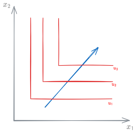
Perfectly complementary goods - 03 - Utility Demand function and Pricing - DME 2024-12-01 13.09.32.excalidraw.png

The arrow represents the direction in which the [[#Utility function]] increases

In this case the [[#Utility function]] is well represented by the [[#Other utility function]].

Undesirable goods

undesirable good

A good is considered undesirable when the consumer does not accept it.

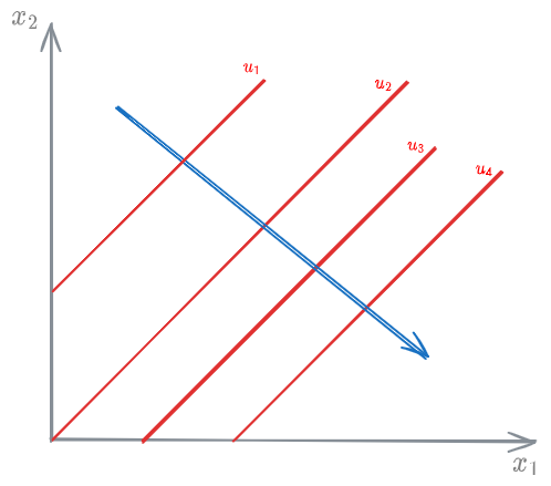
If $x_{2}$ is the undesirable goods, the [[#Utility function]] grows in the direction of decreasing $x_{2}$ and increasing $x_{1}$ .

Undesirable good - 03 - Utility Demand function and Pricing - DME 2024-12-01 13.12.39.excalidraw.png

The arrow represents the direction in which the [[#Utility function]] increases

Demand function

demand function

A demand function ( $x_{i}$ ) is a function that tells how much of a good the customers want:
$x_{i} = f (p_{i}, p_{j}, m)$
where:

$x_{i} :$ Demand of good $i$
$p_{i} :$ Price of good $i$
$p_{j} :$ Price of good different than $i$
$m :$ Budget of the buyer (can be seen as costumer's income)

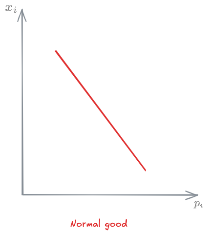
The demand has different patterns depending on the type of good:

%%🖋 Edit in Excalidraw%%

As a function of prices, usually demand decreases as price increases

%%🖋 Edit in Excalidraw%%

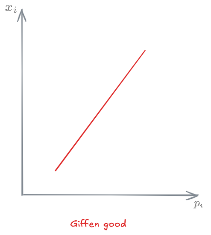
Griffen goods

Giffen goods are goods that, for some reason, have a demand that increases as price increases. This happens for example with some items during emergencies, when there is scarcity (remember face masks during covid).

%%🖋 Edit in Excalidraw%%

Elasticity

In general, finding the [[#Demand function]] is quite difficult. Often times though, we are not really interested in knowing the full demand, but we can work at the local level. We maybe just need to know how the demand varies when changing the several factors. This introduces the concept of elasticity.

demand elasticity ($\varepsilon_{p}$)

Let a demand be $q = f (p)$ .
Elasticity is defined as:
$ε_{p} = lim_{Δ p \to 0} \frac{\frac{Δ q}{q}}{\frac{Δ p}{p}} = \frac{p}{q} \frac{\partial q}{\partial p}$
Elasticity is the ratio between percentage change of demand and price. It tells us how much the demand varies, for a given variation in price (see also Elasticità della domadna).

Types of elasticity

Perfectly elastic demand

perfectly elastic demand

Perfectly elastic demand - 03 - Utility Demand function and Pricing - DME 2024-12-01 16.25.48.excalidraw.png

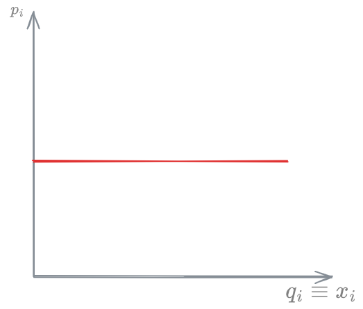
A perfectly elastic demand is one where #Elasticity is infinite:
$ε_{p} = \infty$
This means that, even the slightest change in price will make the demand completely different. Really, what it means is that, even keeping the price constant, makes the demand change freely.

Elastic demand

elastic demand

Elastic demand - 03 - Utility Demand function and Pricing - DME 2024-12-01 16.28.16.excalidraw.png

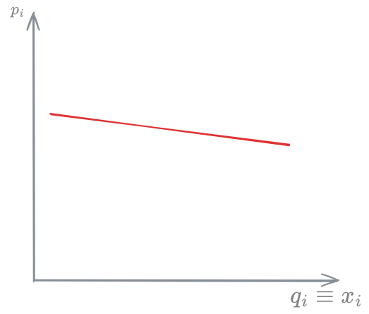
An elastic demand is one where the demand is sensitive to the price. Changing the price strongly affects the demand
$1 < ε_{p} < \infty$

Perfectly inelastic demand

perfectly inelastic demand

Perfectly inelastic demand - 03 - Utility Demand function and Pricing - DME 2024-12-01 16.29.48.excalidraw.png

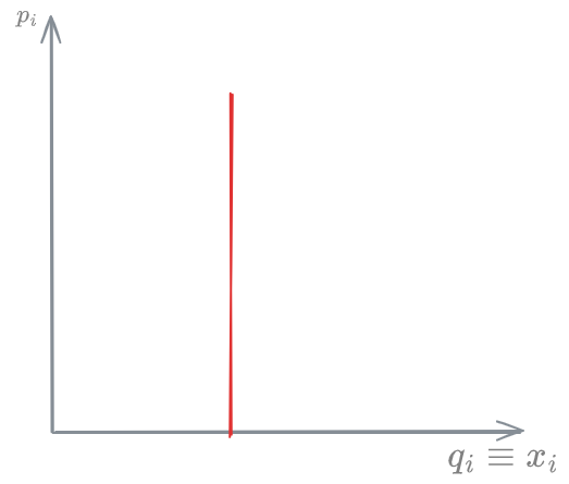
A perfectly inelastic demand is one where for any change in price, the demand stays constant
$ε_{p} = 0$

Inelastic demand

inelastic demand

Inelastic demand - 03 - Utility Demand function and Pricing - DME 2024-12-01 16.32.36.excalidraw.png

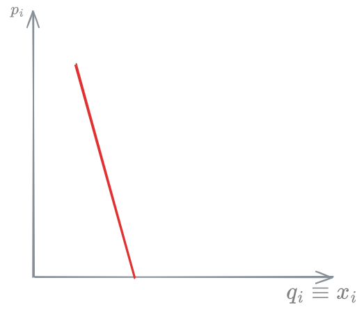
An inelastic demand is one where even big change in prices, only cause small changes in demand.
$0 < ε_{p} < 1$

Unitary elasticity

unitary elasticity

Unitary elasticity - 03 - Utility Demand function and Pricing - DME 2024-12-01 16.34.19.excalidraw.png

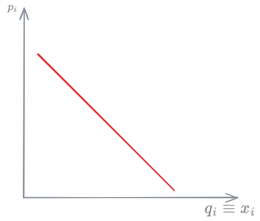
A demand with unitary elasticity is one where for any percentage change in price, the demand changes of the same percentage.
$ε_{p} = 1$

Theory of pricing

Social Welfare is defined as the sum of #Consumer surplus and #Producer surplus

Let's imagine we have the following situation:

A demand ( $q$ ) that increases with the reducing in price
A supply ( $s$ ) that increases with increase in price
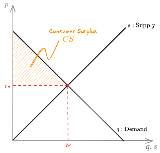
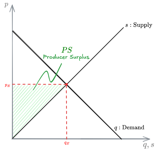
The intersection of the 2 is an equilibrium point, called equilibrium price.

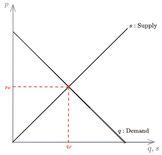
The equilibrium point is how much the costumer/consumer is pays in the current state of the market (with demand $q$ and supply $s$ ).

Notice that, if the producer were to increase the supply, the price would increase. Same if the demand increased. This means that, in reality, the consumer is willing to pay more than $p_{E}$ . The consumer would pay any price indicated by the demand curve $q$ .

Consumer surplus

The consumer surplus is the cumulative amount that all the consumers are still willing to pay given the current market conditions. It's what they're willing to pay on top of what they're paying currently.

In the graph, the consumer suprlus can be seen as the area indicated in orange:

Producer surplus

The producer surplus is the amount of supply that the producer is still willing to provide.

In the graph, is the area in green

Cost, value, price

Let $g$ be the generalized social cost (assuming no externalities):

g = p + c_{u}

where:

$p :$ price
$c_{u} :$ cost (time) of user

From the user prospective we have:

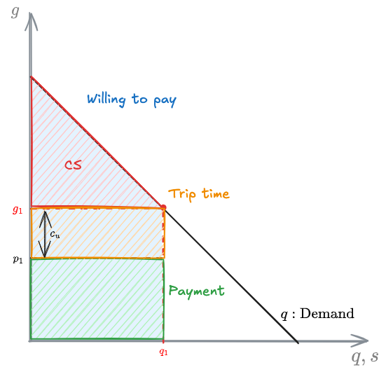
Then, the price costumers are willing to pay at $q_{1}$ is the area in blue:

\int_{0}^{q_{1}} g (z) d z

We can then define:

#Consumer surplus:

C S = \int_{0}^{q_{1}} (g (z) d z) - (p_{1} + c_{u}) q_{1}

CS = Willing to pay - cash - trip time

While, from the producer prospective:

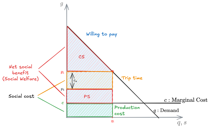
In the graph we have:
The curve $q$ is the demand for a transportation service. Let's imagine we're working with $q_{1}$ users.

The blue area is how much the costumers are cumulatively willing to pay.

The generalized cost for the user will be $g_{1}$

g_{1} = p_{1} + c_{u}

The generalized cost for the user is the sum of the price ( $p_{1}$ ) and all the other external costs (specifically time, $c_{u}$ ).

If it costs the producer $c$ to provide the service, $p_{1} - c$ will be the producer's revenue and the corresponding red area the #Producer surplus.

The total social cost will be the sum of the orange and green areas.
While the net social benefit will be the willing to pay - social cost.

Pricing principles in transportation

Remember that the #Social Welfare is:

S W = C S + P S

The Consumer Surplus is an average cost that mainly depends on the number of users ( $q$ ) and the size of the infrastructure ( $k$ ):

c_{u} (q, k)

The Producer Surplus will depend on:

$r (k) :$ Annual fix cost of the infrastructure
$C^{'} (q) :$ Operating and maintenance costs
$C^{0} (q) :$ Operative cost of vehicles
For simplicity:

C^{'} (q) = c^{'} q C^{0} (q) = c^{0} q

Then, the #Producer surplus is the sum:

\begin{aligned} P S & = C^{0} (q) + C^{'} (q) + r (k) k = \\ = \underset{income}{\underset{⏟}{p q}} \underset{TOT annual costs}{\underset{⏟}{- c^{0} q - c^{'} q - r (k) k}} \end{aligned}

In general, with transportation, we're interested in maximizing the #Social Welfare:

max_{q, k} S W (q, x)

Where the SW:

S W (q, x) = C S (q, k) + P S (q, k)

This, according to what has been said before, can be written as:

\begin{aligned} S W (q, x) & = C S (q, k) + P S (q, k) = \\ = \int_{0}^{q_{1}} (g (z) d z) - c_{u} (q, k) q - c^{0} q - c^{'} q - r (k) k \end{aligned}

where notice that, the term $- p q$ for the PS is already in the CS. We don't have to count this twice (this is clearer looking at the graph)

S W (q, x) = \int_{0}^{q_{1}} (g (z) d z) - c_{u} (q, k) q - c^{0} q - c^{'} q - r (k) k

To maximize this function, we calculate the first derivatives (in $q$ and $k$ ) and impose it equal to 0:

\begin{aligned} \frac{\partial}{\partial q} S W (q, x) = g (q) - c_{u} (q, k) - \frac{\partial c_{u} (q, k)}{\partial q} q - c^{0} - c^{'} & \overset{!}{=} 0 ⟶ q^{*} [1] \\ \frac{\partial}{\partial k} S W (q, x) = - q \frac{\partial c_{u} (q, k)}{\partial k} - r (k) - \frac{\partial r (k)}{\partial k} k & \overset{!}{=} 0 ⟶ k^{*} [2] \end{aligned}

Now, $[1]$ can be written as:

g (q^{*}) = c_{u} (q^{*}, k) + {\frac{\partial c_{u} (q, k)}{\partial q} |}_{q^{*}} q^{*} + c^{0} + c^{'}

And, remembering the definition of generalized cost:

g = p + c_{u} (q, k)

we can write:

c_{u} (q, k) + \underset{Social Marginal cost}{\underset{⏟}{\frac{\partial c_{u} (q, k)}{\partial q}}} q + c^{0} + c^{'} = p + c_{u} (q, k)

So:

p = c^{0} + c^{'} + q^{*} {\frac{\partial c_{u}}{\partial q} |}_{q^{*}, k^{*}}

❗❗❗❗❗❗❗❗❗❗❗❗
❗❗❗ COMPLETARE ❗❗❗
❗❗❗❗❗❗❗❗❗❗❗❗

03 - Utility Demand function and Pricing - DME

Utility function

Properties of the utility function

Types of utility function

Cobb-Douglas utility function

Quasilinear utility function

Linear utility function

Other utility function

Indifference curve

Budget constrain

Theory of election

Relation of Marginal Substitution

Particular cases

Perfectly substitutive goods

Perfectly complementary goods

Undesirable goods

Demand function

Griffen goods

Elasticity

Types of elasticity

Perfectly elastic demand

Elastic demand

Perfectly inelastic demand

Inelastic demand

Unitary elasticity

Theory of pricing

Social Welfare

Consumer surplus

Producer surplus

Cost, value, price

Pricing principles in transportation

Maximizing the social welfare

Pricing without congestion