01 - Production and cost functions in transport - DME
01 - Production and cost functions in transport - DME
Production function
The production function is the relation between the output (products,
It works under the assumption of efficient process: given
Indicators
Average Productivity
Marginal Productivity
Marginal productivity is a measure of how many units of input are necessary to increase the output of 1 unit.
Characteristics
Usually, a #Production function tends to have the following characteristics:
Monotony of a production function
The #Production function increases when the labor or the capital increases, or, at the very least, it stays constant. It NEVER decreases.
Convexity of a production function
The product
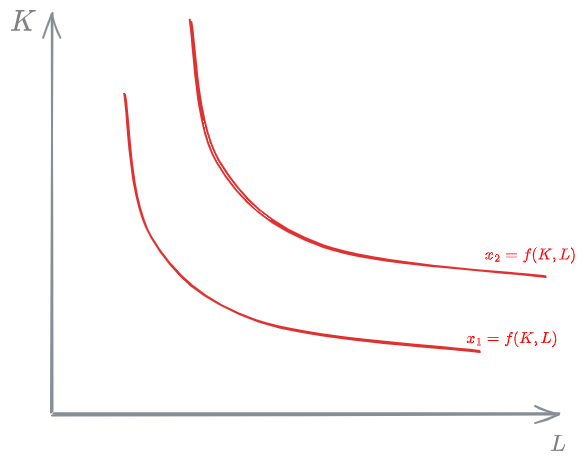
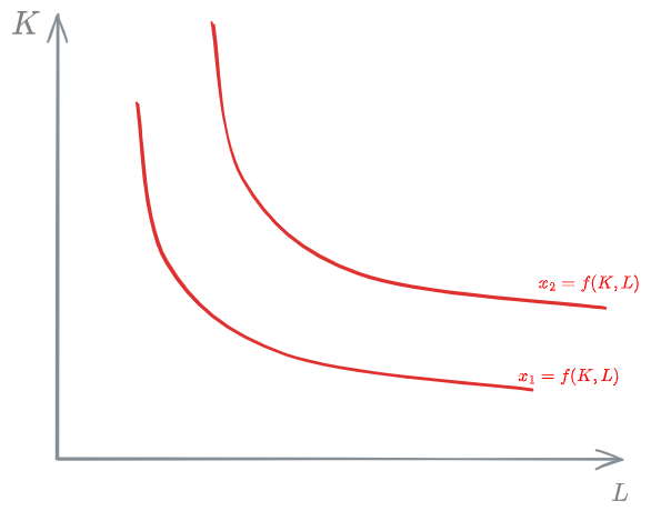
Iso-production curves
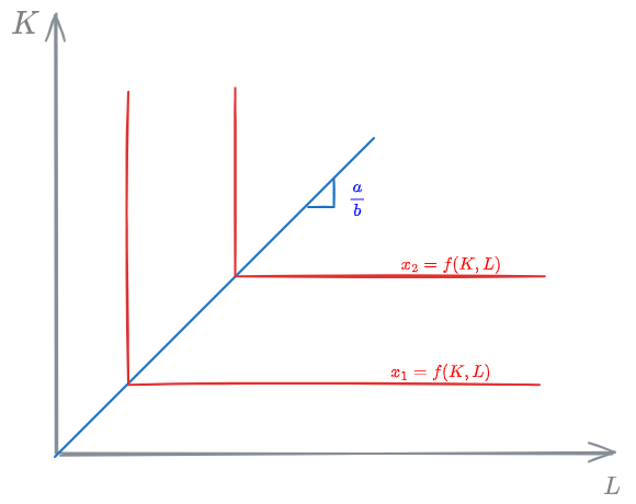
They show what are the admissible combinations of labor and capital for a given value of the [[#Production function]].
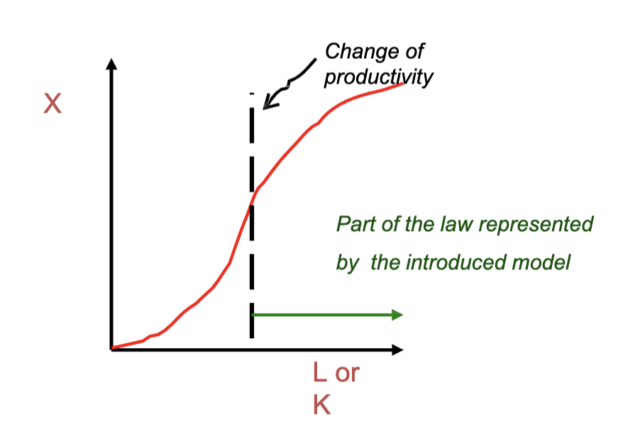
Diminishing return law
Assuming a production function
Return to scale
Return to scale is the concept of relating how fast the [[#Production function]] increases with the increase of the inputs:
- [[#Increasing return to scale]]
- [[#Constant return to scale]]
- [[#Reducing return to scale]]
Increasing return to scale
We have an increasing return to scale when the [[#Production function]] increases more than proportionally with the inputs.
Keeping in mind that the production function is [[Homogenous Function]] (like the cost function), we have in creasing return to scale if:
Constant return to scale
We have a constant return to scale when the [[#Production function]] increases proportionally with the inputs.
Reducing return to scale
We have a reducing return to scale when the [[#Production function]] increases less than proportionally with the inputs.
Types of production function
There are a few [[#Iso-production curves]] that are often used in the field:
- [[#Cobb-Douglas]]
- [[#Leontief]]
Cobb-Douglas
The Cobb-Douglas [[#Iso-production curves]] has the following equation for the [[#Production function]]
where:
are 2 parameters
The Cobb-Douglas function can be written linearly:
In the Cobb-Douglas function, the [[#Return to scale]] is:
Leontief
The Leontief [[#Production function]] is often used for its simplicity:
Technical Substitution Relation (TSR)
- [?] I don't understand what Technical substitution relation is?
The iso-production curve below is given:
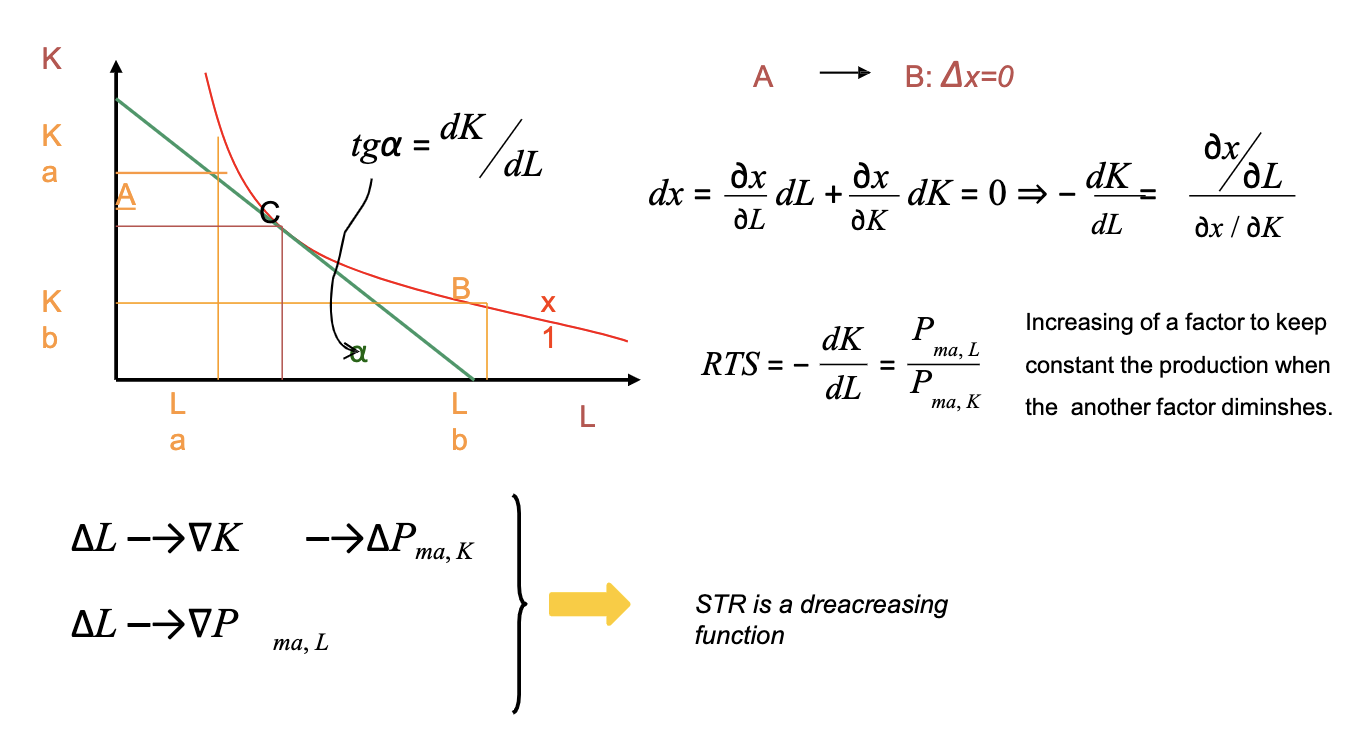
By definition, along the curve,
The differential of
meaning we can write:
where, at the second member, we recognize the marginal productivities:
This last quantity is defined as Technical Substitution Relation
Technical Substitution Relation (
Cost Function
[[01 - Production and cost functions in transport - DME]]
The Cost Function, or Total cost (
where:
number of productive factors unitary cost of the productive factors
We work under the assumption that we have the minimum cost for producing
Indicators
Average cost
Marginal cost
Properties of the cost function
???
There is no diminishing with unitary cost of the productive factors
Homogeneity of the cost function
The #Cost Function is homogeneous of first grade in
Convexity of the cost function
The #Cost Function is convex in
Continuity of the cost function
The #Cost Function is continous in
Fixed and variable costs
The total cost can be divided into the following sum:
where
[[#Fixed cost]] [[#Variable cost]]
Fixed cost
Fixed costs (
Variable cost
Variable costs (
They exist both in the #Short term cost function and the #Long term cost function.
Short term and long term
Short term cost function
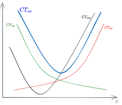
In the short term, the [[#Cost Function]] is given by the sum of the [[#Variable cost]] and the [[#Fixed cost]]:
The graph specifically shows the sum of the Average Fixed cost and the Average Variable cost to give, in blue, the [[#Average cost]].
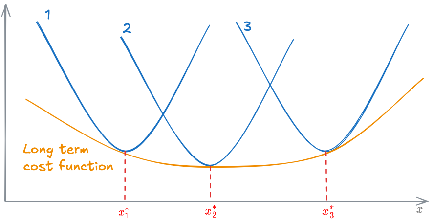
Long term cost function
In the long term, even the [[#Fixed cost]] can change. Therefore, there are not [[#Fixed cost]] in the Long term cost function, only [[#Variable cost]].
The long term cost function can be obtained overlapping all the [[#Short term cost function]] at different sizes of the system:
Each
Efficiency
Efficiency is the condition where we get the maximum output for a fixed numer of productive factors.
Types of efficiency
We can define efficiency based on different things:
- [[#Technical efficiency]]
- [[#Efficiency of market assignation]]
- [[#Social efficiency]]
- [[#Efficiency of scale]]
- [[#Structural Efficiency]]
Technical efficiency
Technical efficiency is reached when the cost is minimized.
Efficiency of market assignation
When efficient market decisions are made.
Social efficiency
Social efficiency is the #Efficiency condition when Externalities are included.
Efficiency of scale
Current capacity vs ideal capacity
- Ideal: combination of inputs and outputs inside the constant returns to scale
- Long-term competitive equilibrium, where production has constant returns to scale
Structural Efficiency
Structural efficiency is reached when production is located in the non-congested region of possibile inputs combinations.
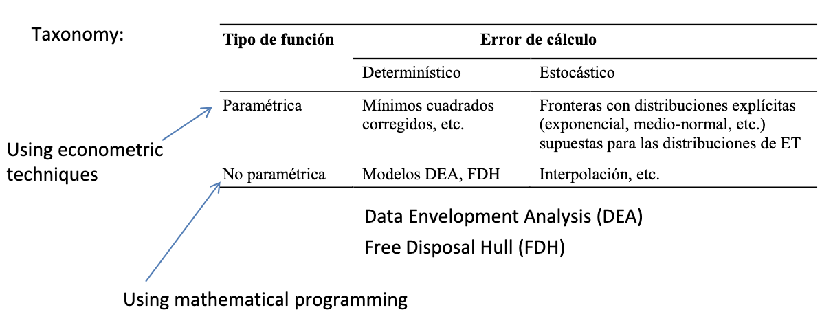
How to measure efficiency
Economy of scale
[[#Average cost]]
If the nature of a business is to take advantage of economy of scale, that business will try to grow. There will then be just a few big businesses in that sector.
Economy of density
Economy of density is the concept in which a business sees its cost decreasing when the density of the business increases.
The total cost to transport passengers decreases by increasing utilisation of existing vehicle fleet and infrastructure capacity within a market area of given size.
Mohring effect
The Mohring effect is a scenario where, adding users to a transportation network actually decreases the average cost incurred by the user.
Let's try to understand this through an example:
Imagine we have a road. Every time another car enters the road, the road becomes more conjested and travel time increases for every one. This is a normal behavior.
Let's consider now a bus line. An increase in users will make the ride more unconfortable for everyone, since the bus will be more crowded. At a certain point though, if there are enough users, the bus company might decide to add more buses increasing the ferquency. This will shorten travel time for everyone and increase everyone's comfort. In this case, an increase in users has reduced the average cost incurred by each user. This last one, was an example of the Mohring effect.

